Curve Fitting Least Squares Regression Chapter 17 1

~ Curve Fitting ~ Least Squares Regression Chapter 17 1 Copyright © 2006 The Mc. Graw-Hill Companies, Inc. Permission required for reproduction or display.

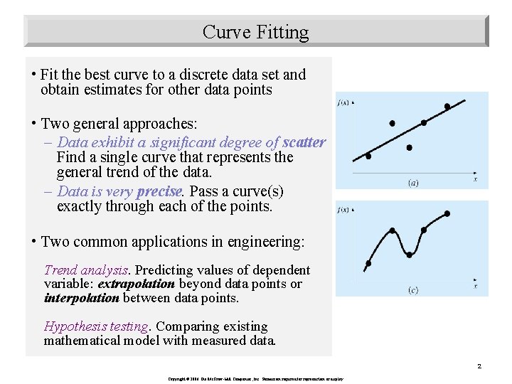
Curve Fitting • Fit the best curve to a discrete data set and obtain estimates for other data points • Two general approaches: – Data exhibit a significant degree of scatter Find a single curve that represents the general trend of the data. – Data is very precise. Pass a curve(s) exactly through each of the points. • Two common applications in engineering: Trend analysis. Predicting values of dependent variable: extrapolation beyond data points or interpolation between data points. Hypothesis testing. Comparing existing mathematical model with measured data. 2 Copyright © 2006 The Mc. Graw-Hill Companies, Inc. Permission required for reproduction or display.

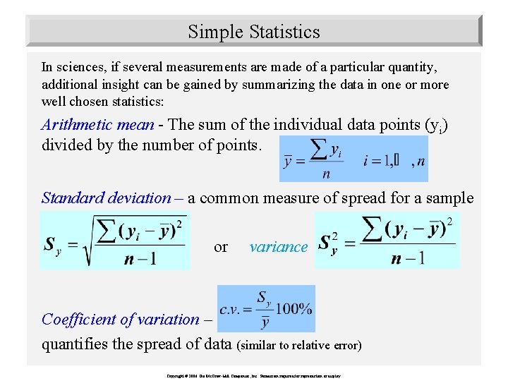
Simple Statistics In sciences, if several measurements are made of a particular quantity, additional insight can be gained by summarizing the data in one or more well chosen statistics: Arithmetic mean - The sum of the individual data points (yi) divided by the number of points. Standard deviation – a common measure of spread for a sample or variance Coefficient of variation – quantifies the spread of data (similar to relative error) 3 Copyright © 2006 The Mc. Graw-Hill Companies, Inc. Permission required for reproduction or display.

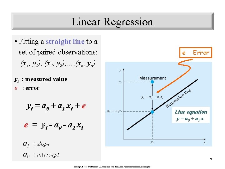
Linear Regression • Fitting a straight line to a set of paired observations: (x 1, y 1), (x 2, y 2), …, (xn, yn) e Error yi : measured value e : error yi = a 0 + a 1 xi + e e = yi - a 0 - a 1 xi a 1 : slope a 0 : intercept Line equation y = a 0 + a 1 x 4 Copyright © 2006 The Mc. Graw-Hill Companies, Inc. Permission required for reproduction or display.

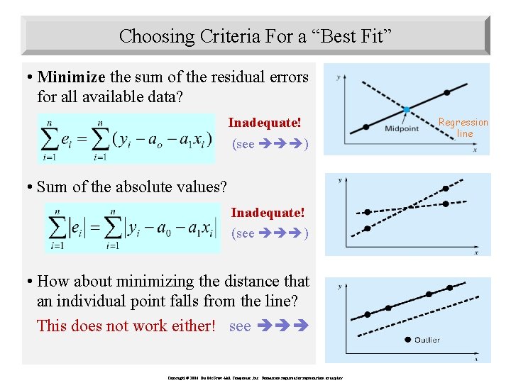
Choosing Criteria For a “Best Fit” • Minimize the sum of the residual errors for all available data? Inadequate! (see ) • Sum of the absolute values? Inadequate! (see ) • How about minimizing the distance that an individual point falls from the line? This does not work either! see Copyright © 2006 The Mc. Graw-Hill Companies, Inc. Permission required for reproduction or display. Regression line

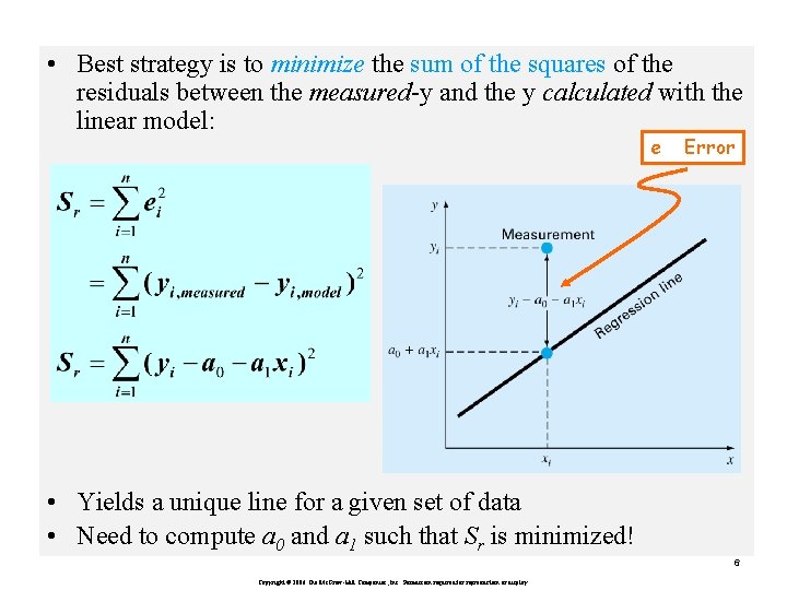
• Best strategy is to minimize the sum of the squares of the residuals between the measured-y and the y calculated with the linear model: e Error • Yields a unique line for a given set of data • Need to compute a 0 and a 1 such that Sr is minimized! 6 Copyright © 2006 The Mc. Graw-Hill Companies, Inc. Permission required for reproduction or display.

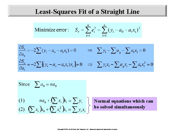
Least-Squares Fit of a Straight Line Normal equations which can be solved simultaneously Copyright © 2006 The Mc. Graw-Hill Companies, Inc. Permission required for reproduction or display.

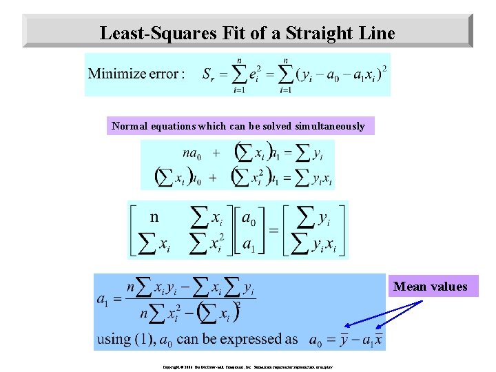
Least-Squares Fit of a Straight Line Normal equations which can be solved simultaneously Mean values Copyright © 2006 The Mc. Graw-Hill Companies, Inc. Permission required for reproduction or display.

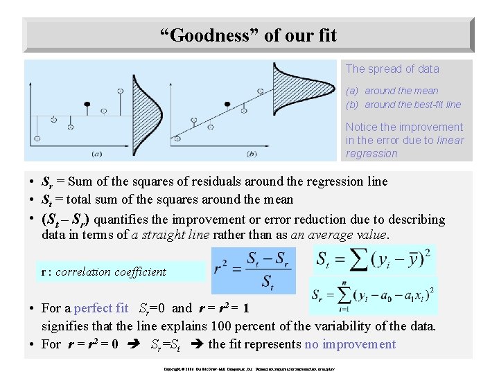
“Goodness” of our fit The spread of data (a) around the mean (b) around the best-fit line Notice the improvement in the error due to linear regression • Sr = Sum of the squares of residuals around the regression line • St = total sum of the squares around the mean • (St – Sr) quantifies the improvement or error reduction due to describing data in terms of a straight line rather than as an average value. r : correlation coefficient • For a perfect fit Sr=0 and r = r 2 = 1 signifies that the line explains 100 percent of the variability of the data. • For r = r 2 = 0 Sr=St the fit represents no improvement Copyright © 2006 The Mc. Graw-Hill Companies, Inc. Permission required for reproduction or display.

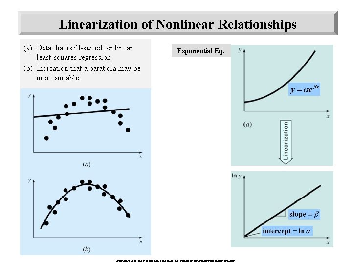
Linearization of Nonlinear Relationships (a) Data that is ill-suited for linear least-squares regression (b) Indication that a parabola may be more suitable Exponential Eq. Copyright © 2006 The Mc. Graw-Hill Companies, Inc. Permission required for reproduction or display.

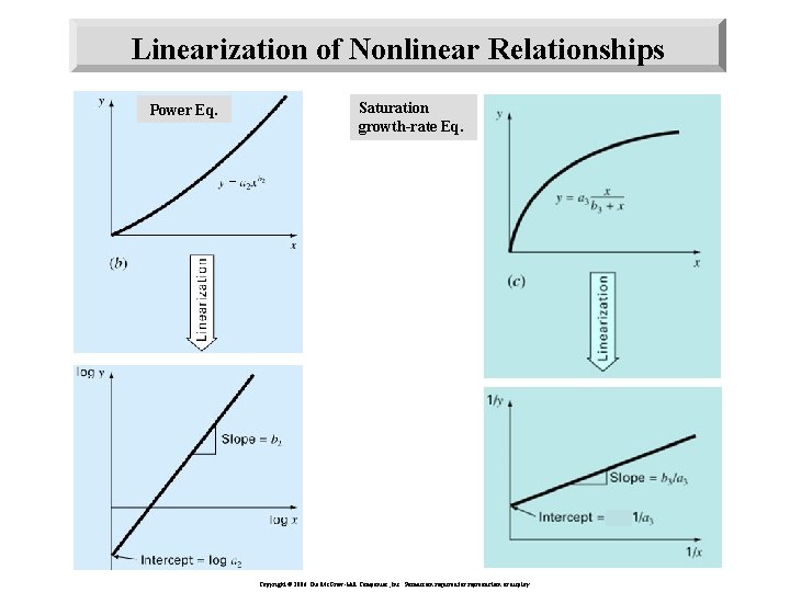
Linearization of Nonlinear Relationships Power Eq. Saturation growth-rate Eq. Copyright © 2006 The Mc. Graw-Hill Companies, Inc. Permission required for reproduction or display.

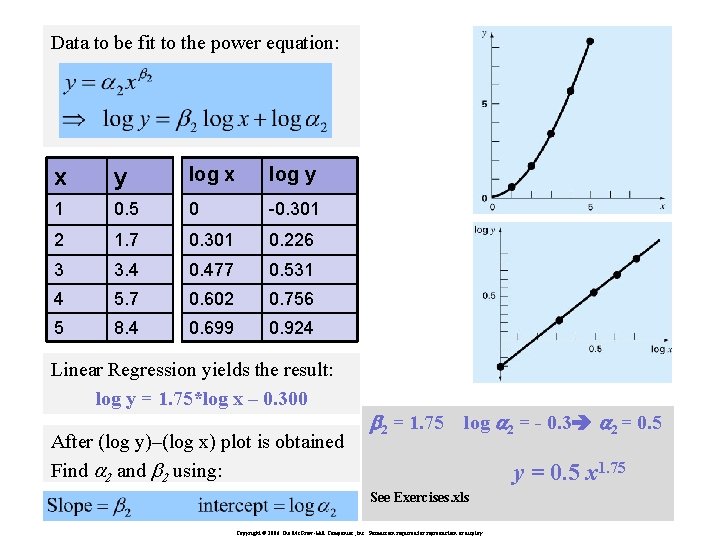
Data to be fit to the power equation: x y log x log y 1 0. 5 0 -0. 301 2 1. 7 0. 301 0. 226 3 3. 4 0. 477 0. 531 4 5. 7 0. 602 0. 756 5 8. 4 0. 699 0. 924 Linear Regression yields the result: log y = 1. 75*log x – 0. 300 After (log y)–(log x) plot is obtained Find a 2 and b 2 using: b 2 = 1. 75 log a 2 = - 0. 3 a 2 = 0. 5 y = 0. 5 x 1. 75 See Exercises. xls Copyright © 2006 The Mc. Graw-Hill Companies, Inc. Permission required for reproduction or display.

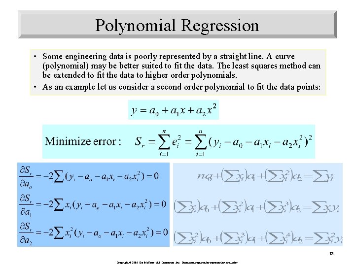
Polynomial Regression • Some engineering data is poorly represented by a straight line. A curve (polynomial) may be better suited to fit the data. The least squares method can be extended to fit the data to higher order polynomials. • As an example let us consider a second order polynomial to fit the data points: 13 Copyright © 2006 The Mc. Graw-Hill Companies, Inc. Permission required for reproduction or display.

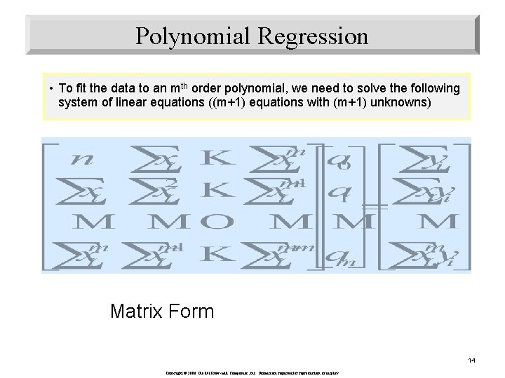
Polynomial Regression • To fit the data to an mth order polynomial, we need to solve the following system of linear equations ((m+1) equations with (m+1) unknowns) Matrix Form 14 Copyright © 2006 The Mc. Graw-Hill Companies, Inc. Permission required for reproduction or display.

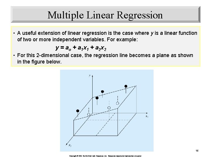
Multiple Linear Regression • A useful extension of linear regression is the case where y is a linear function of two or more independent variables. For example: y = a o + a 1 x 1 + a 2 x 2 • For this 2 -dimensional case, the regression line becomes a plane as shown in the figure below. 15 Copyright © 2006 The Mc. Graw-Hill Companies, Inc. Permission required for reproduction or display.

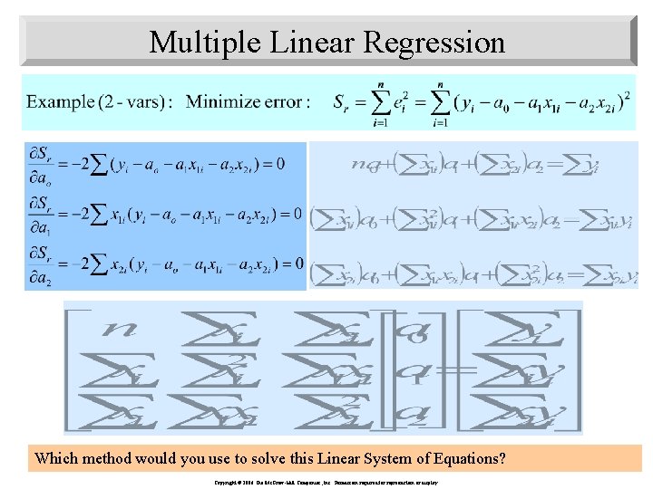
Multiple Linear Regression Which method would you use to solve this Linear System of Equations? Copyright © 2006 The Mc. Graw-Hill Companies, Inc. Permission required for reproduction or display. 16

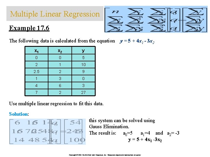
Multiple Linear Regression Example 17. 6 The following data is calculated from the equation x 1 x 2 y 0 0 5 2 1 10 2. 5 2 9 1 3 0 4 6 3 7 2 27 y = 5 + 4 x 1 - 3 x 2 Use multiple linear regression to fit this data. Solution: this system can be solved using Gauss Elimination. The result is: a 0=5 a 1=4 and a 2= -3 y = 5 + 4 x 1 -3 x 2 Copyright © 2006 The Mc. Graw-Hill Companies, Inc. Permission required for reproduction or display.