LESSON 1 INVENTORY MODELS STOCHASTIC Outline SinglePeriod Models

LESSON 1: INVENTORY MODELS (STOCHASTIC) Outline • Single-Period Models – Discrete Demand – Continuous Demand, Uniform Distribution – Continuous Demand, Normal Distribution • Multi-Period Models – Given a Q, R Policy, Find Cost – Optimal Q, R Policy without Service Constraint – Optimal Q, R Policy with Type 1 Service Constraint – Optimal Q, R Policy with Type 2 Service Constraint

Stochastic Inventory Control Models Inventory Control with Uncertain Demand • In Lessons 16 -20 we shall discuss the stochastic inventory control models assuming that the exact demand is not known. However, some demand characteristics such as mean, standard deviation and the distribution of demand are assumed to be known. • Penalty cost, : Shortages occur when the demand exceeds the amount of inventory on hand. For each unit of unfulfilled demand, a penalty cost of is charged. One source of penalty cost is the loss of profit. For example, if an item is purchased at $1. 50 and sold at $3. 00, the loss of profit is $3. 00 -1. 50 = $1. 50 for each unit of demand not fulfilled.

Stochastic Inventory Control Models Inventory Control with Uncertain Demand • More on penalty cost, – Penalty cost is estimated differently in different situation. There are two cases: 1. Backorder - if the excess demand is backlogged and fulfilled in a future period, a backorder cost is charged. Backorder cost is estimated from bookkeeping, delay costs, goodwill etc. 2. Lost sales - if the excess demand is lost because the customer goes elsewhere, the lost sales is charged. The lost sales include goodwill and loss of profit margin. So, penalty cost = selling price - unit variable cost + goodwill, if there exists any goodwill.

Single- and Multi- Period Models • Stochastic models are classified into single- and multiperiod models. • In a single-period model, items are received in the beginning of a period and sold during the same period. The unsold items are not carried over to the next period. • The unsold items may be a total waste, or sold at a reduced price, or returned to the producer at some price less than the original purchase price. • The revenue generated by the unsold items is called the salvage value.

Single- and Multi- Period Models • Following are some products for which a single-period model may be appropriate: – Computer that will be obsolete before the next order – Perishable products – Seasonal products such as bathing suits, winter coats, etc. – Newspaper and magazine • In the single-period model, there remains only one question to answer: how much to order.

Single- and Multi- Period Models • In a multi-period model, all the items unsold at the end of one period are available in the next period. • If in a multi-period model orders are placed at regular intervals e. g. , once a week, once a month, etc, then there is only one question to answer: how much to order. • However, we discuss Q, R models in which it is assumed that an order may be placed anytime. So, as usual, there are two questions: how much to order and when to order.

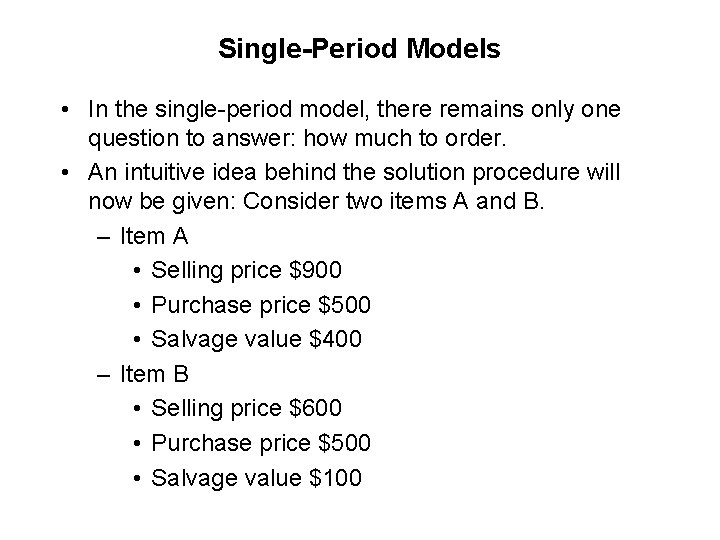
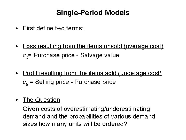
Single-Period Models • In the single-period model, there remains only one question to answer: how much to order. • An intuitive idea behind the solution procedure will now be given: Consider two items A and B. – Item A • Selling price $900 • Purchase price $500 • Salvage value $400 – Item B • Selling price $600 • Purchase price $500 • Salvage value $100

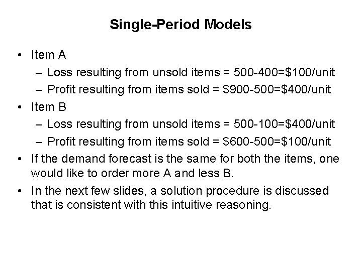
Single-Period Models • Item A – Loss resulting from unsold items = 500 -400=$100/unit – Profit resulting from items sold = $900 -500=$400/unit • Item B – Loss resulting from unsold items = 500 -100=$400/unit – Profit resulting from items sold = $600 -500=$100/unit • If the demand forecast is the same for both the items, one would like to order more A and less B. • In the next few slides, a solution procedure is discussed that is consistent with this intuitive reasoning.

Single-Period Models • First define two terms: • Loss resulting from the items unsold (overage cost) co= Purchase price - Salvage value • Profit resulting from the items sold (underage cost) cu = Selling price - Purchase price • The Question Given costs of overestimating/underestimating demand the probabilities of various demand sizes how many units will be ordered?

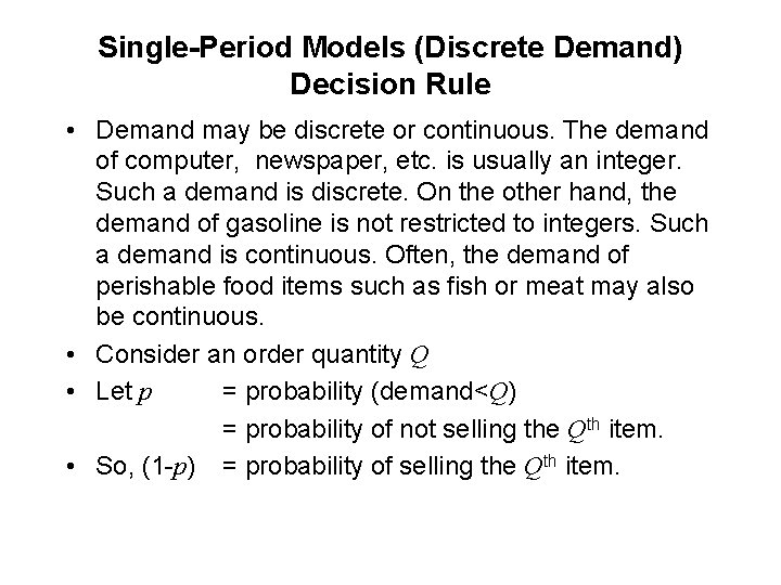
Single-Period Models (Discrete Demand) Decision Rule • Demand may be discrete or continuous. The demand of computer, newspaper, etc. is usually an integer. Such a demand is discrete. On the other hand, the demand of gasoline is not restricted to integers. Such a demand is continuous. Often, the demand of perishable food items such as fish or meat may also be continuous. • Consider an order quantity Q • Let p = probability (demand<Q) = probability of not selling the Qth item. • So, (1 -p) = probability of selling the Qth item.

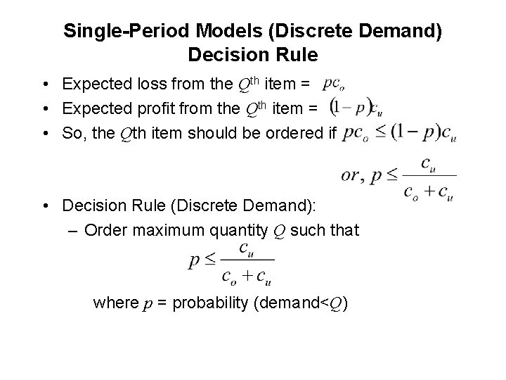
Single-Period Models (Discrete Demand) Decision Rule • Expected loss from the Qth item = • Expected profit from the Qth item = • So, the Qth item should be ordered if • Decision Rule (Discrete Demand): – Order maximum quantity Q such that where p = probability (demand<Q)

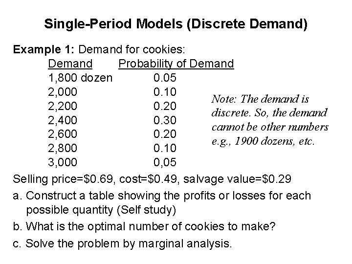
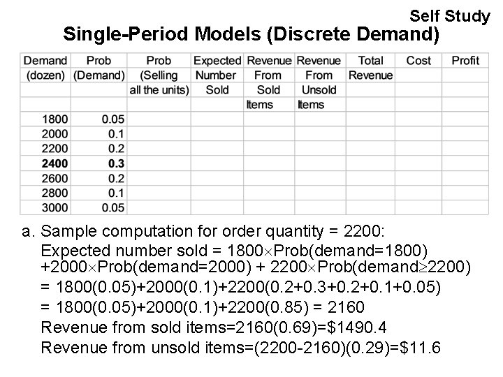
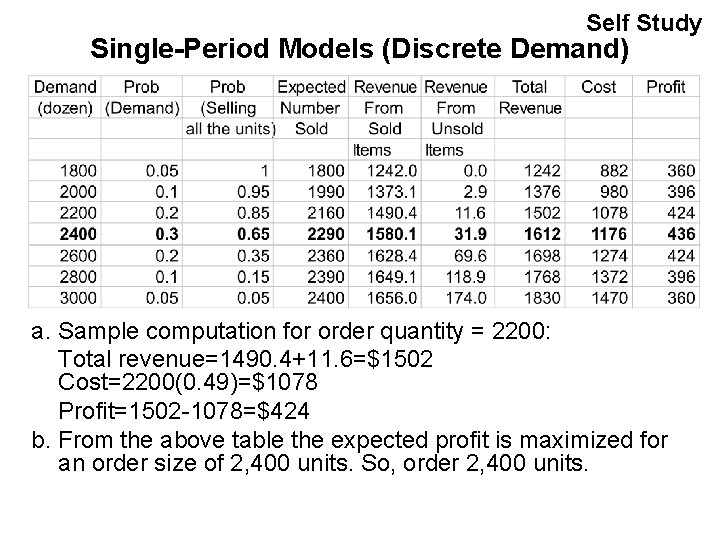
Single-Period Models (Discrete Demand) Example 1: Demand for cookies: Demand Probability of Demand 1, 800 dozen 0. 05 2, 000 0. 10 Note: The demand is 2, 200 0. 20 discrete. So, the demand 2, 400 0. 30 cannot be other numbers 2, 600 0. 20 e. g. , 1900 dozens, etc. 2, 800 0. 10 3, 000 0, 05 Selling price=$0. 69, cost=$0. 49, salvage value=$0. 29 a. Construct a table showing the profits or losses for each possible quantity (Self study) b. What is the optimal number of cookies to make? c. Solve the problem by marginal analysis.

Self Study Single-Period Models (Discrete Demand) a. Sample computation for order quantity = 2200: Expected number sold = 1800 Prob(demand=1800) +2000 Prob(demand=2000) + 2200 Prob(demand 2200) = 1800(0. 05)+2000(0. 1)+2200(0. 2+0. 3+0. 2+0. 1+0. 05) = 1800(0. 05)+2000(0. 1)+2200(0. 85) = 2160 Revenue from sold items=2160(0. 69)=$1490. 4 Revenue from unsold items=(2200 -2160)(0. 29)=$11. 6

Self Study Single-Period Models (Discrete Demand) a. Sample computation for order quantity = 2200: Total revenue=1490. 4+11. 6=$1502 Cost=2200(0. 49)=$1078 Profit=1502 -1078=$424 b. From the above table the expected profit is maximized for an order size of 2, 400 units. So, order 2, 400 units.

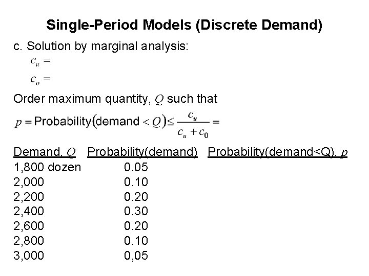
Single-Period Models (Discrete Demand) c. Solution by marginal analysis: Order maximum quantity, Q such that Demand, Q Probability(demand) Probability(demand<Q), p 1, 800 dozen 0. 05 2, 000 0. 10 2, 200 0. 20 2, 400 0. 30 2, 600 0. 20 2, 800 0. 10 3, 000 0, 05

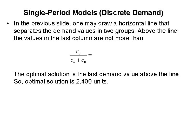
Single-Period Models (Discrete Demand) • In the previous slide, one may draw a horizontal line that separates the demand values in two groups. Above the line, the values in the last column are not more than The optimal solution is the last demand value above the line. So, optimal solution is 2, 400 units.

Continuous Distribution • Often the demand is continuous. Even when the demand is not continuous, continuous distribution may be used because the discrete distribution may be inconvenient. • For example, suppose that the demand of calendar can vary between 150 to 850 units. If demand varies so widely, a continuous approximation is more convenient because discrete distribution will involve a large number of computation without any significant increase in accuracy. • We shall discuss two distributions: – Uniform distribution – Continuous distribution

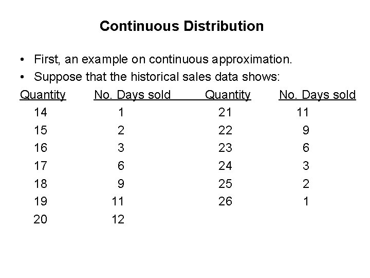
Continuous Distribution • First, an example on continuous approximation. • Suppose that the historical sales data shows: Quantity No. Days sold 14 1 21 11 15 2 22 9 16 3 23 6 17 6 24 3 18 9 25 2 19 11 26 1 20 12

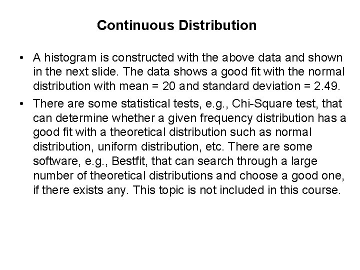
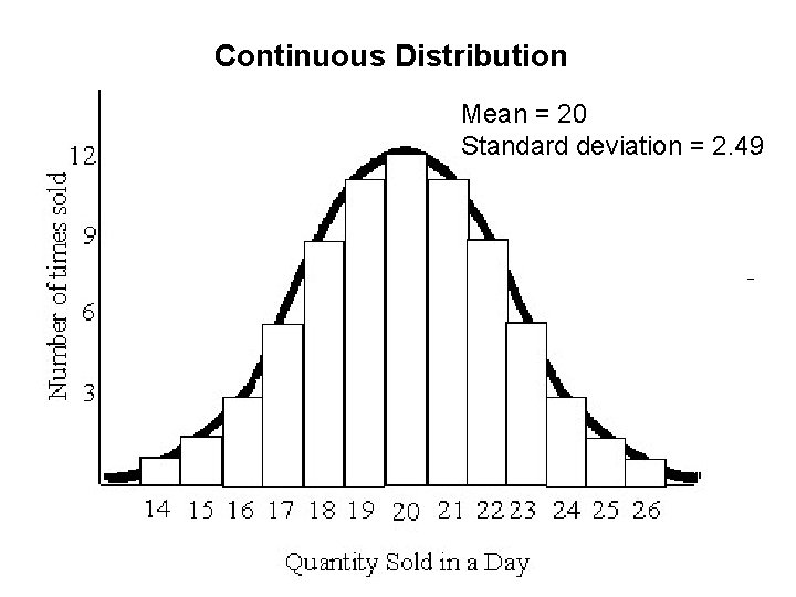
Continuous Distribution • A histogram is constructed with the above data and shown in the next slide. The data shows a good fit with the normal distribution with mean = 20 and standard deviation = 2. 49. • There are some statistical tests, e. g. , Chi-Square test, that can determine whether a given frequency distribution has a good fit with a theoretical distribution such as normal distribution, uniform distribution, etc. There are some software, e. g. , Bestfit, that can search through a large number of theoretical distributions and choose a good one, if there exists any. This topic is not included in this course.

Continuous Distribution Mean = 20 Standard deviation = 2. 49

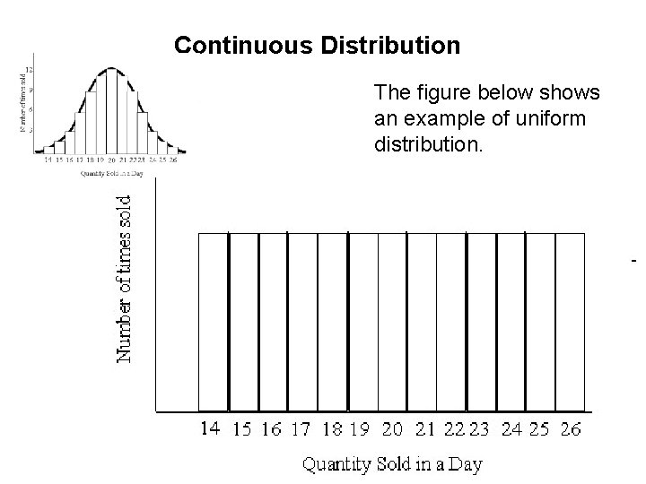
Continuous Distribution The figure below shows an example of uniform distribution.

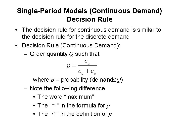
Single-Period Models (Continuous Demand) Decision Rule • The decision rule for continuous demand is similar to the decision rule for the discrete demand • Decision Rule (Continuous Demand): – Order quantity Q such that where p = probability (demand Q) – Note the following difference • The word “maximum” • The “= “ in the formula for p • The “ “ in the definition of p

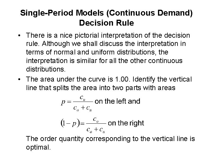
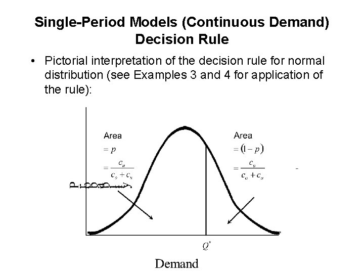
Single-Period Models (Continuous Demand) Decision Rule • There is a nice pictorial interpretation of the decision rule. Although we shall discuss the interpretation in terms of normal and uniform distributions, the interpretation is similar for all the other continuous distributions. • The area under the curve is 1. 00. Identify the vertical line that splits the area into two parts with areas The order quantity corresponding to the vertical line is optimal.

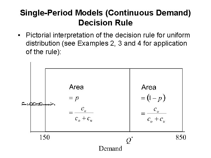
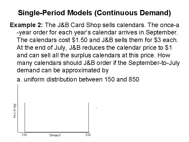
Single-Period Models (Continuous Demand) Decision Rule • Pictorial interpretation of the decision rule for uniform distribution (see Examples 2, 3 and 4 for application of the rule):

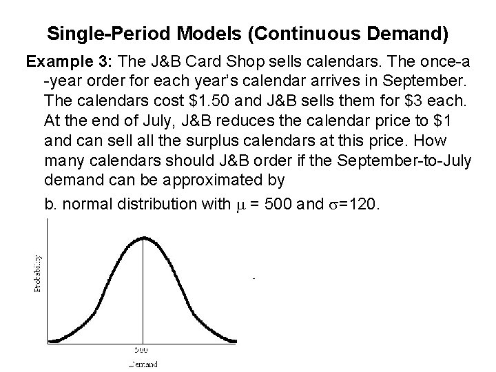
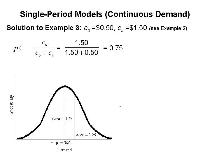
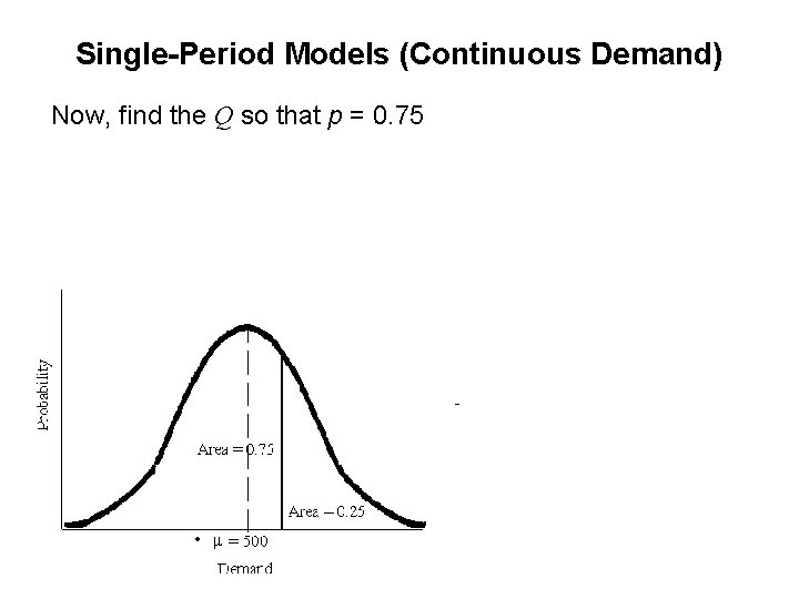
Single-Period Models (Continuous Demand) Decision Rule • Pictorial interpretation of the decision rule for normal distribution (see Examples 3 and 4 for application of the rule):

Single-Period Models (Continuous Demand) Example 2: The J&B Card Shop sells calendars. The once-a -year order for each year’s calendar arrives in September. The calendars cost $1. 50 and J&B sells them for $3 each. At the end of July, J&B reduces the calendar price to $1 and can sell all the surplus calendars at this price. How many calendars should J&B order if the September-to-July demand can be approximated by a. uniform distribution between 150 and 850

Single-Period Models (Continuous Demand) Solution to Example 2: Overage cost co = Purchase price - Salvage value = Underage cost cu = Selling price - Purchase price =

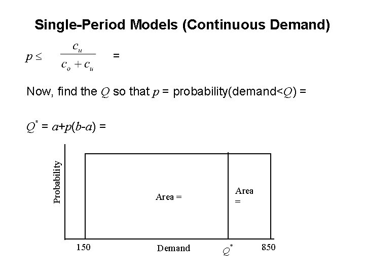
Single-Period Models (Continuous Demand) = p Now, find the Q so that p = probability(demand<Q) = Probability Q* = a+p(b-a) = Area = 150 Demand Q* 850

Single-Period Models (Continuous Demand) Example 3: The J&B Card Shop sells calendars. The once-a -year order for each year’s calendar arrives in September. The calendars cost $1. 50 and J&B sells them for $3 each. At the end of July, J&B reduces the calendar price to $1 and can sell all the surplus calendars at this price. How many calendars should J&B order if the September-to-July demand can be approximated by b. normal distribution with = 500 and =120.

Single-Period Models (Continuous Demand) Solution to Example 3: co =$0. 50, cu =$1. 50 (see Example 2) p = = 0. 75

Single-Period Models (Continuous Demand) Now, find the Q so that p = 0. 75

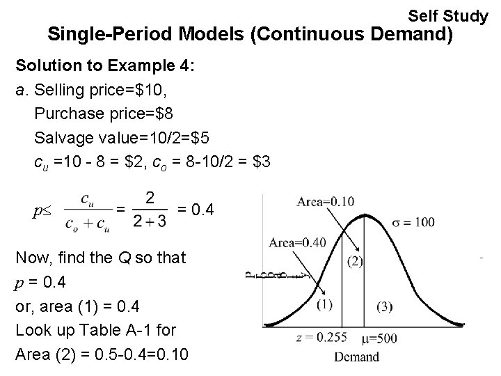
Self Study Single-Period Models (Continuous Demand) Example 4: A retail outlet sells a seasonal product for $10 per unit. The cost of the product is $8 per unit. All units not sold during the regular season are sold for half the retail price in an end-of-season clearance sale. Assume that the demand for the product is normally distributed with = 500 and = 100. a. What is the recommended order quantity? b. What is the probability of a stockout? c. To keep customers happy and returning to the store later, the owner feels that stockouts should be avoided if at all possible. What is your recommended quantity if the owner is willing to tolerate a 0. 15 probability of stockout? d. Using your answer to part (c), what is the goodwill cost you are assigning to a stockout?

Self Study Single-Period Models (Continuous Demand) Solution to Example 4: a. Selling price=$10, Purchase price=$8 Salvage value=10/2=$5 cu =10 - 8 = $2, co = 8 -10/2 = $3 p = = 0. 4 Now, find the Q so that p = 0. 4 or, area (1) = 0. 4 Look up Table A-1 for Area (2) = 0. 5 -0. 4=0. 10

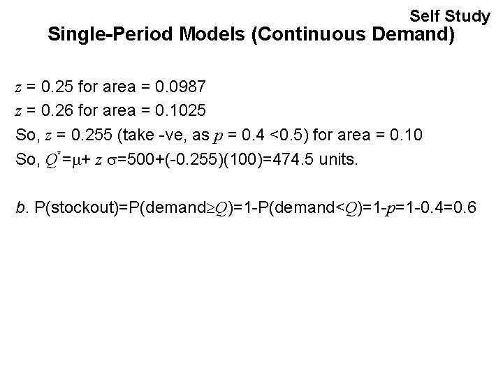
Self Study Single-Period Models (Continuous Demand) z = 0. 25 for area = 0. 0987 z = 0. 26 for area = 0. 1025 So, z = 0. 255 (take -ve, as p = 0. 4 <0. 5) for area = 0. 10 So, Q*= + z =500+(-0. 255)(100)=474. 5 units. b. P(stockout)=P(demand Q)=1 -P(demand<Q)=1 -p=1 -0. 4=0. 6

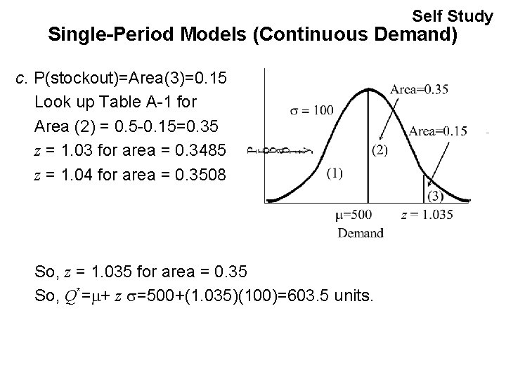
Self Study Single-Period Models (Continuous Demand) c. P(stockout)=Area(3)=0. 15 Look up Table A-1 for Area (2) = 0. 5 -0. 15=0. 35 z = 1. 03 for area = 0. 3485 z = 1. 04 for area = 0. 3508 So, z = 1. 035 for area = 0. 35 So, Q*= + z =500+(1. 035)(100)=603. 5 units.

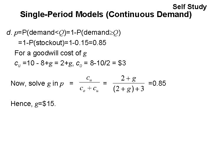
Self Study Single-Period Models (Continuous Demand) d. p=P(demand<Q)=1 -P(demand Q) =1 -P(stockout)=1 -0. 15=0. 85 For a goodwill cost of g cu =10 - 8+g = 2+g, co = 8 -10/2 = $3 Now, solve g in p = Hence, g=$15. = =0. 85

READING AND EXERCISES Lesson 1 Reading: Section 5. 1 - 5. 3 , pp. 245 -254 (4 th Ed. ), pp. 232 -245 (5 th Ed. ) Exercise: 8 a, 12 a, and 12 b, pp. 256 -258 (4 th Ed. ), pp. 248 -250 (5 th Ed. )

LESSON 2: INVENTORY MODELS (STOCHASTIC) INTRODUCTION TO THE Q, R SYSTEMS Outline • Multi-Period Models – Lot size-Reorder Point (Q, R) Systems – Notation, Definition and Some Formula – Example: Given a Q, R Policy, Find Cost

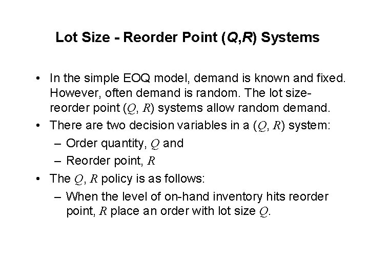
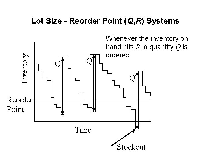
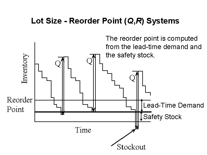
Lot Size - Reorder Point (Q, R) Systems • In the simple EOQ model, demand is known and fixed. However, often demand is random. The lot sizereorder point (Q, R) systems allow random demand. • There are two decision variables in a (Q, R) system: – Order quantity, Q and – Reorder point, R • The Q, R policy is as follows: – When the level of on-hand inventory hits reorder point, R place an order with lot size Q.

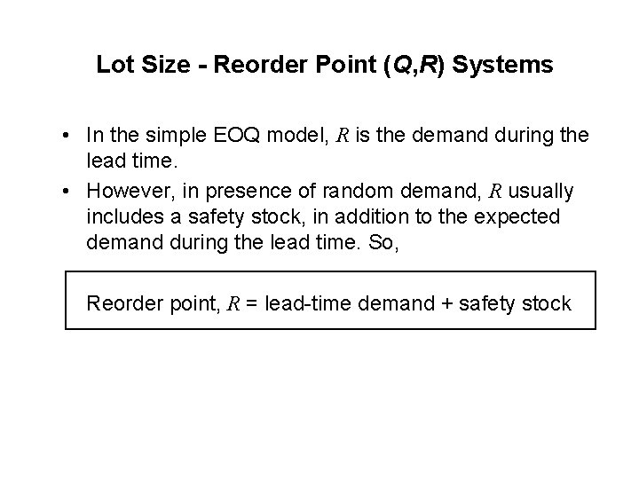
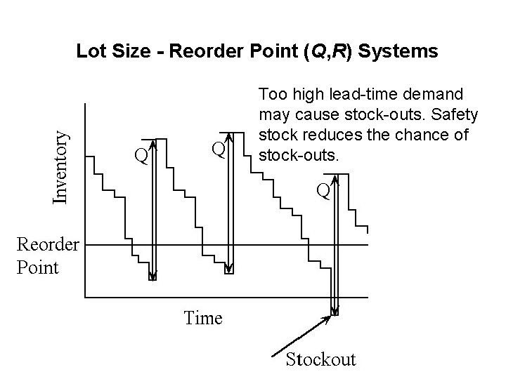
Lot Size - Reorder Point (Q, R) Systems • In the simple EOQ model, R is the demand during the lead time. • However, in presence of random demand, R usually includes a safety stock, in addition to the expected demand during the lead time. So, Reorder point, R = lead-time demand + safety stock

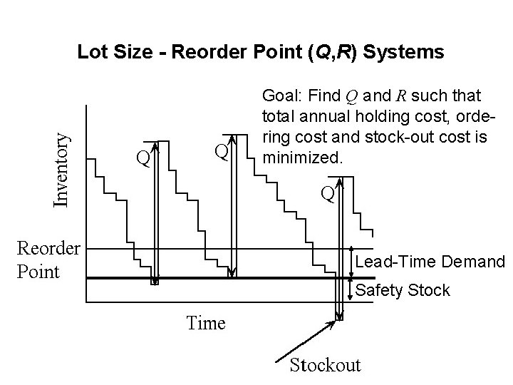
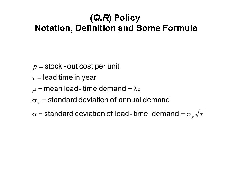
Lot Size - Reorder Point (Q, R) Systems • In the simple EOQ model, only holding cost and ordering costs are considered. • In presence of random demand, the demand may sometimes be too high and exceed the inventory on hand. The result is stock-out. • For each unit of shortage, a penalty cost p is charged. See Lesson 16 for more information on penalty cost. Penalty cost = p per unit.

Lot Size - Reorder Point (Q, R) Systems • The goal of a lot size-reorder point system is to find Q and R so that the total annual holding cost, ordering cost and stock-out cost is minimized. • The current lesson only covers how to compute cost from a given policy. • The next three lessons address the question how to find optimal Q and R so that the total annual cost is minimized.

Lot Size - Reorder Point (Q, R) Systems Whenever the inventory on hand hits R, a quantity Q is ordered.

Lot Size - Reorder Point (Q, R) Systems Too high lead-time demand may cause stock-outs. Safety stock reduces the chance of stock-outs.

Lot Size - Reorder Point (Q, R) Systems The reorder point is computed from the lead-time demand the safety stock. Lead-Time Demand Safety Stock

Lot Size - Reorder Point (Q, R) Systems Goal: Find Q and R such that total annual holding cost, ordering cost and stock-out cost is minimized. Lead-Time Demand Safety Stock

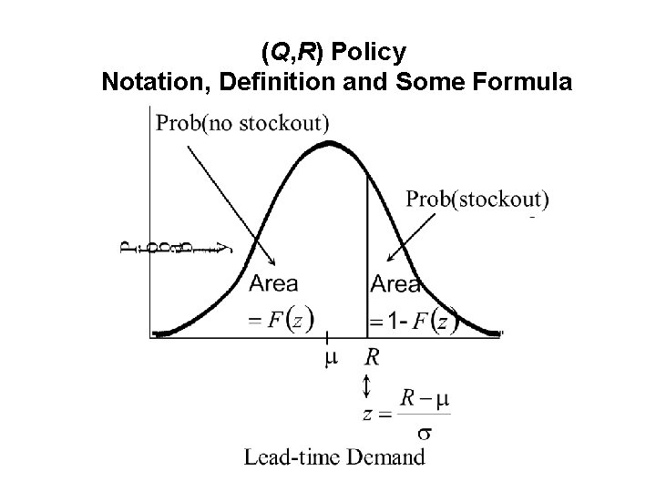
(Q, R) Policy Notation, Definition and Some Formula

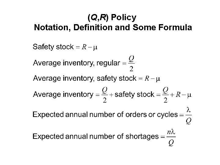
(Q, R) Policy Notation, Definition and Some Formula

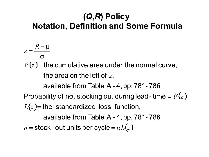
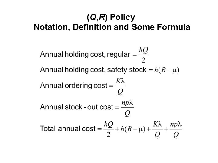
(Q, R) Policy Notation, Definition and Some Formula

(Q, R) Policy Notation, Definition and Some Formula

(Q, R) Policy Notation, Definition and Some Formula

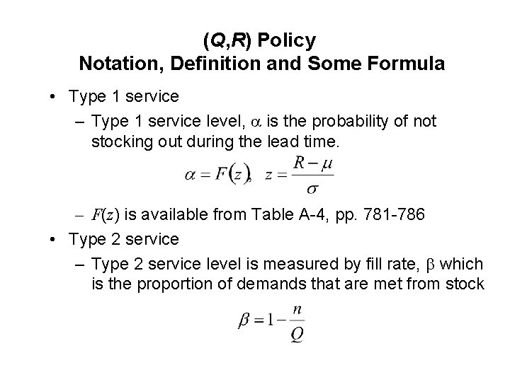
(Q, R) Policy Notation, Definition and Some Formula • Type 1 service – Type 1 service level, is the probability of not stocking out during the lead time. – F(z) is available from Table A-4, pp. 781 -786 • Type 2 service – Type 2 service level is measured by fill rate, which is the proportion of demands that are met from stock

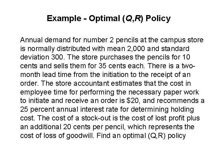
Example - Given A Q, R Policy, Find Cost Annual demand for number 2 pencils at the campus store is normally distributed with mean 2, 000 and standard deviation 300. The store purchases the pencils for 10 cents and sells them for 35 cents each. There is a twomonth lead time from the initiation to the receipt of an order. The store accountant estimates that the cost in employee time for performing the necessary paper work to initiate and receive an order is $20, and recommends a 25 percent annual interest rate for determining holding cost. The cost of a stock-out is the cost of lost profit plus an additional 20 cents per pencil, which represents the cost of loss of goodwill. Currently, a (Q, R) system with Q = 1500, R = 500 is used.

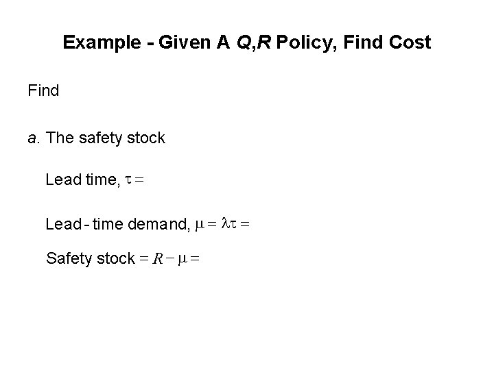
Example - Given A Q, R Policy, Find Cost Find a. The safety stock Lead time, t = Lead - time demand, = lt = Safety stock = R - =

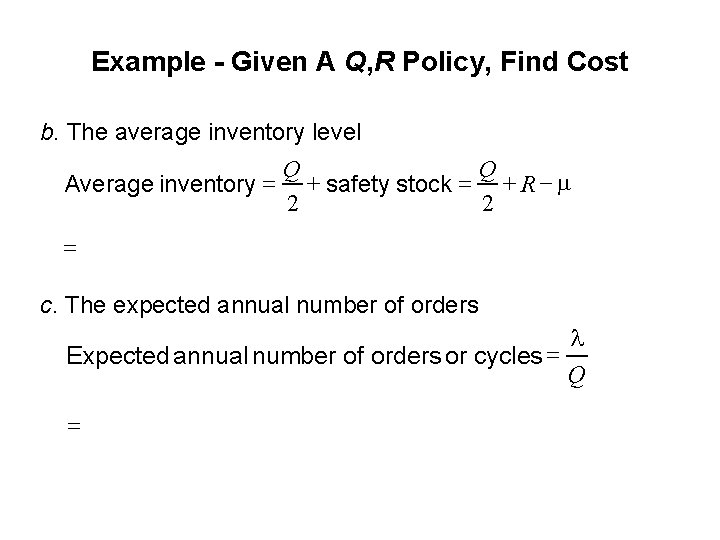
Example - Given A Q, R Policy, Find Cost b. The average inventory level Average inventory = Q Q + safety stock = + R - 2 2 = c. The expected annual number of orders l Expected annual number of orders or cycles = Q =

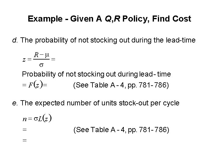
Example - Given A Q, R Policy, Find Cost d. The probability of not stocking out during the lead-time R - = z= Probability of not stocking out during lead - time = F (z ) = (See Table A - 4, pp. 781 - 786) e. The expected number of units stock-out per cycle n = L(z ) = = (See Table A - 4, pp. 781 - 786)

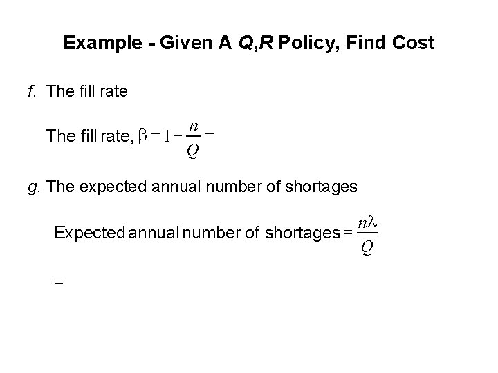
Example - Given A Q, R Policy, Find Cost f. The fill rate, = 1 - n = Q g. The expected annual number of shortages nl Expected annual number of shortages = Q =

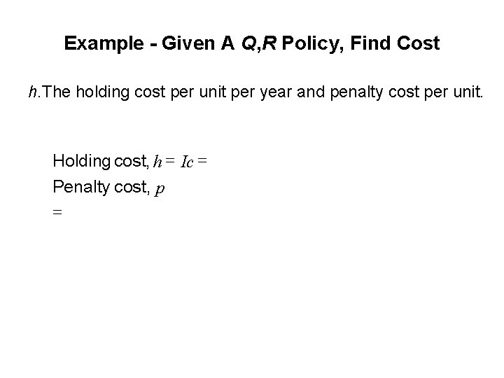
Example - Given A Q, R Policy, Find Cost h. The holding cost per unit per year and penalty cost per unit. Holding cost, h = Ic = Penalty cost, p =

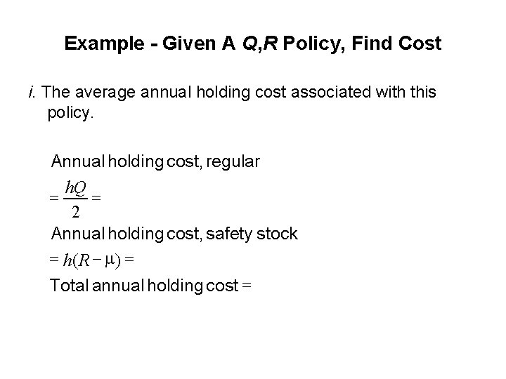
Example - Given A Q, R Policy, Find Cost i. The average annual holding cost associated with this policy. Annual holding cost, regular h. Q = = 2 Annual holding cost, safety stock = h( R - ) = Total annual holding cost =

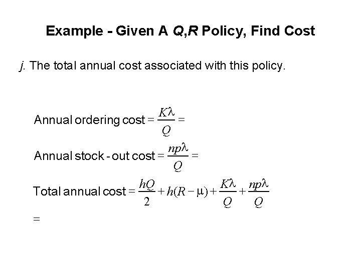
Example - Given A Q, R Policy, Find Cost j. The total annual cost associated with this policy. Kl = Annual ordering cost = Q npl = Annual stock - out cost = Q h. Q Kl npl + h( R - ) + + Total annual cost = 2 Q Q =

READING AND EXERCISES Lesson 2 Reading: Section 5. 4, pp. 259 -262 (4 th Ed. ), pp. 250 -254 (5 th Ed. ) Exercise: 13 b (use the result of 13 a), p. 271 (4 th Ed. ), p. 261 (5 th Ed. )

LESSON 3: INVENTORY MODELS (STOCHASTIC) Q, R SYSTEMS OPTIMIZATION WITHOUT SERVICE Outline • Multi-Period Models – Lot size-Reorder Point (Q, R) Systems • Optimization without service – Procedure – Example

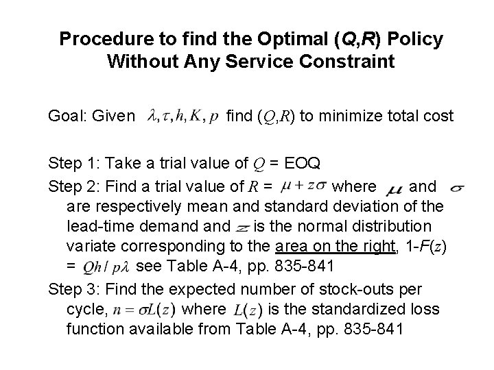
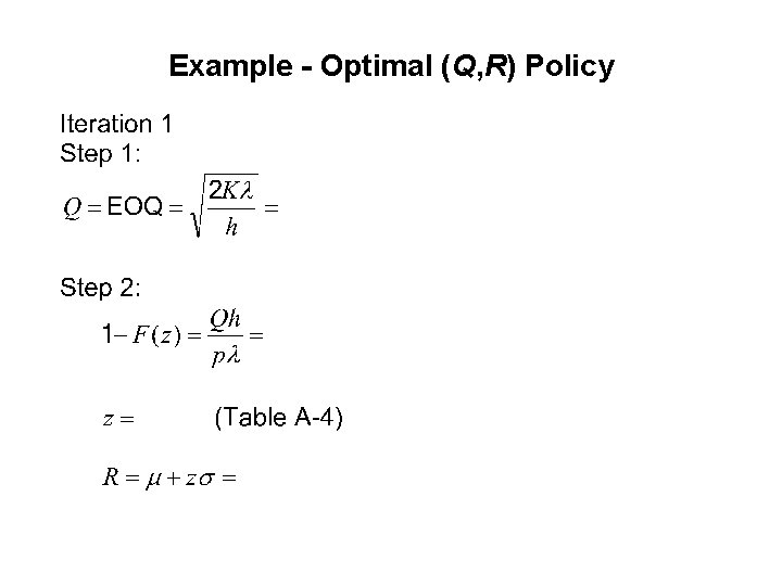
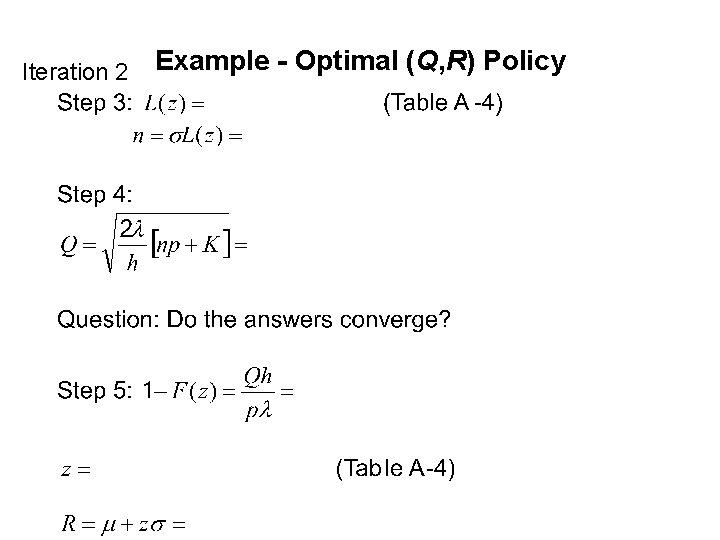
Procedure to find the Optimal (Q, R) Policy Without Any Service Constraint Goal: Given find (Q, R) to minimize total cost Step 1: Take a trial value of Q = EOQ Step 2: Find a trial value of R = where and are respectively mean and standard deviation of the lead-time demand is the normal distribution variate corresponding to the area on the right, 1 -F(z) = see Table A-4, pp. 835 -841 Step 3: Find the expected number of stock-outs per cycle, where is the standardized loss function available from Table A-4, pp. 835 -841

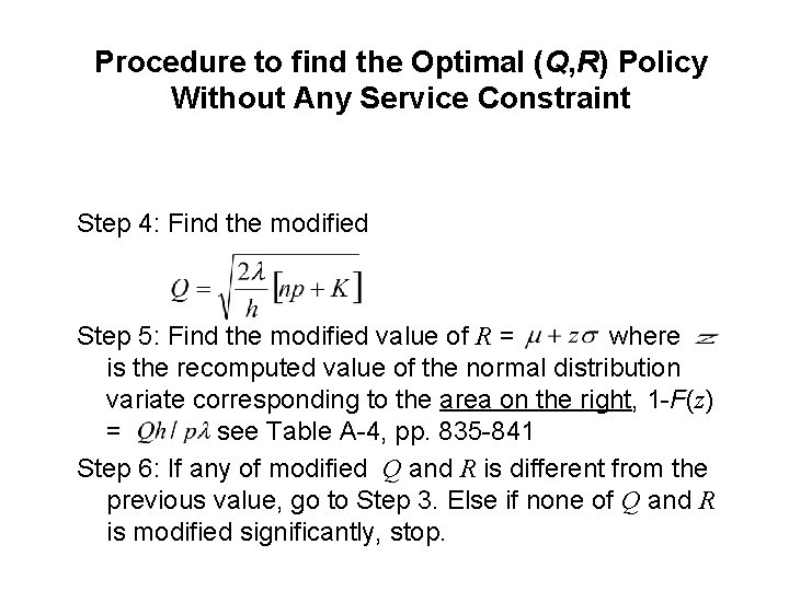
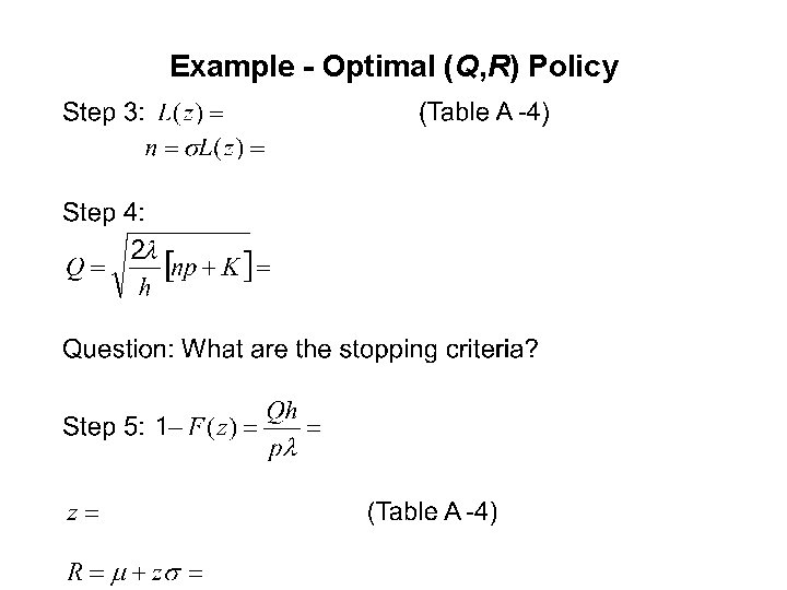
Procedure to find the Optimal (Q, R) Policy Without Any Service Constraint Step 4: Find the modified Step 5: Find the modified value of R = where is the recomputed value of the normal distribution variate corresponding to the area on the right, 1 -F(z) = see Table A-4, pp. 835 -841 Step 6: If any of modified Q and R is different from the previous value, go to Step 3. Else if none of Q and R is modified significantly, stop.

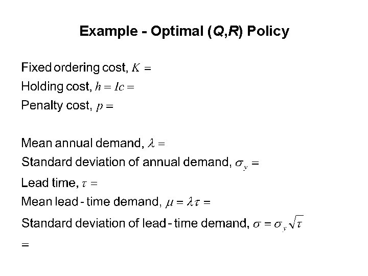
Example - Optimal (Q, R) Policy Annual demand for number 2 pencils at the campus store is normally distributed with mean 2, 000 and standard deviation 300. The store purchases the pencils for 10 cents and sells them for 35 cents each. There is a twomonth lead time from the initiation to the receipt of an order. The store accountant estimates that the cost in employee time for performing the necessary paper work to initiate and receive an order is $20, and recommends a 25 percent annual interest rate for determining holding cost. The cost of a stock-out is the cost of lost profit plus an additional 20 cents per pencil, which represents the cost of loss of goodwill. Find an optimal (Q, R) policy

Example - Optimal (Q, R) Policy

Example - Optimal (Q, R) Policy

Example - Optimal (Q, R) Policy

Iteration 2 Example - Optimal (Q, R) Policy

READING AND EXERCISES Lesson 3 Reading: Section 5. 4, pp. 262 -264 (4 th Ed. ), pp. 253 -255 (5 th Ed. ) Exercise: 13 a, p. 271 (4 th Ed. ), p. 261

LESSON 4: INVENTORY MODELS (STOCHASTIC) Q, R SYSTEMS OPTIMIZATION WITH SERVICE Outline • Multi-Period Models – Lot size-Reorder Point (Q, R) Systems • Optimization with service – Procedure for Type 1 Service – Procedure for Type 2 Service – Example

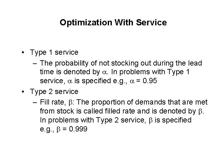
Optimization With Service • In Lesson 18, we discuss the procedure of finding an optimal Q, R policy without any service constraint and using a stock-out penalty cost of p per unit. • Managers often have difficulties to estimate p. • A substitute for stock-out penalty cost, p. is service level. • In this lesson we shall not use stock-out penalty cost, p. Instead , we shall assume that a service level must be met. Next slide defines two major types of service levels.

Optimization With Service • Type 1 service – The probability of not stocking out during the lead time is denoted by . In problems with Type 1 service, is specified e. g. , = 0. 95 • Type 2 service – Fill rate, : The proportion of demands that are met from stock is called filled rate and is denoted by . In problems with Type 2 service, is specified e. g. , = 0. 999

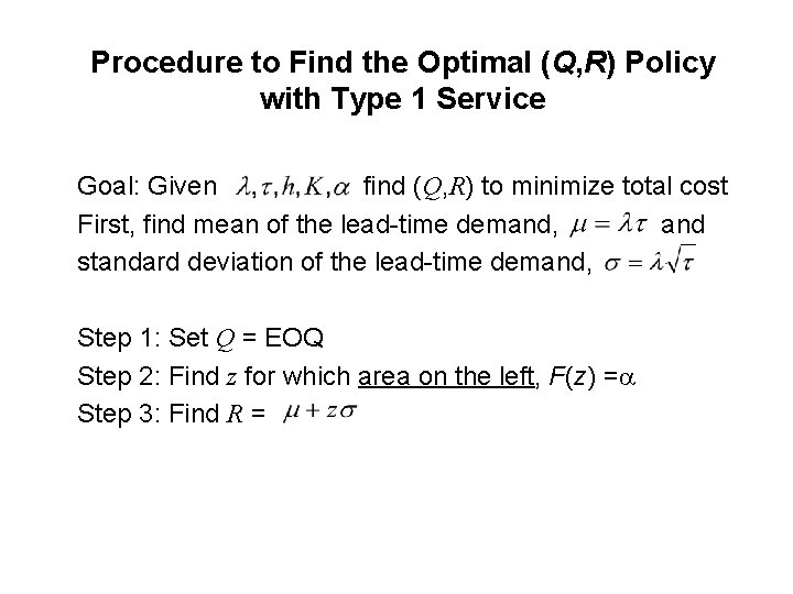
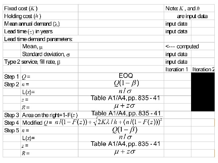
Procedure to Find the Optimal (Q, R) Policy with Type 1 Service Goal: Given find (Q, R) to minimize total cost First, find mean of the lead-time demand, and standard deviation of the lead-time demand, Step 1: Set Q = EOQ Step 2: Find z for which area on the left, F(z) = Step 3: Find R =

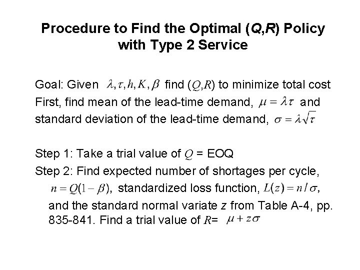
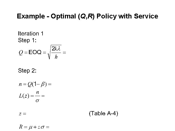
Procedure to Find the Optimal (Q, R) Policy with Type 2 Service Goal: Given find (Q, R) to minimize total cost First, find mean of the lead-time demand, and standard deviation of the lead-time demand, Step 1: Take a trial value of Q = EOQ Step 2: Find expected number of shortages per cycle, standardized loss function, and the standard normal variate z from Table A-4, pp. 835 -841. Find a trial value of R=

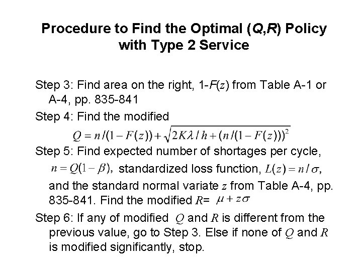
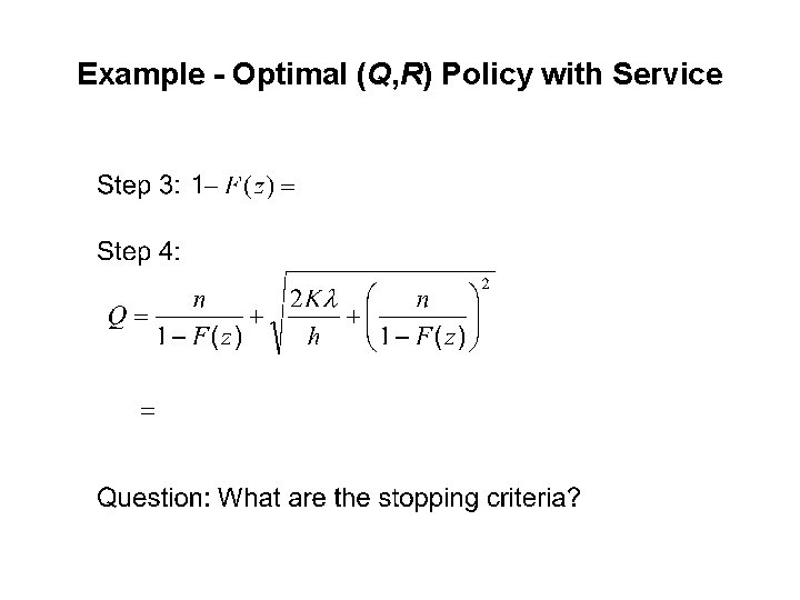
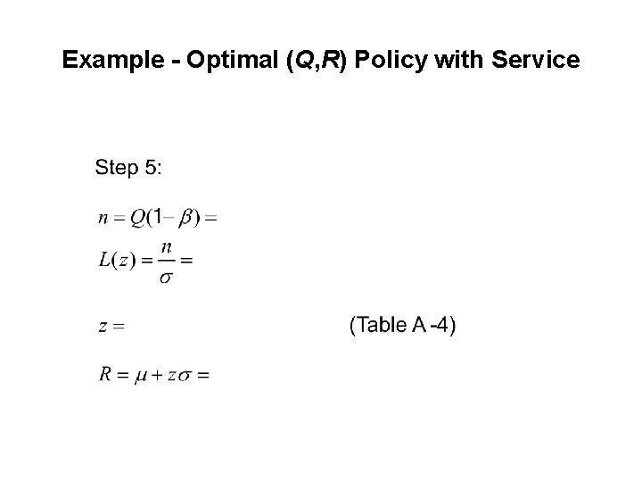
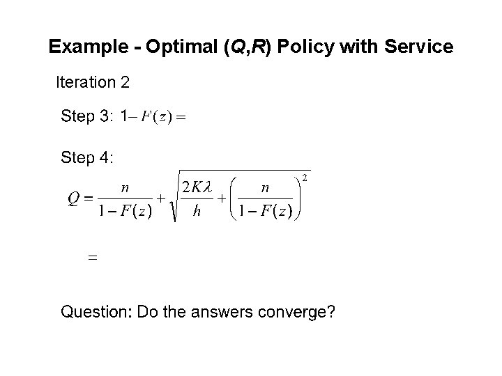
Procedure to Find the Optimal (Q, R) Policy with Type 2 Service Step 3: Find area on the right, 1 -F(z) from Table A-1 or A-4, pp. 835 -841 Step 4: Find the modified Step 5: Find expected number of shortages per cycle, standardized loss function, and the standard normal variate z from Table A-4, pp. 835 -841. Find the modified R= Step 6: If any of modified Q and R is different from the previous value, go to Step 3. Else if none of Q and R is modified significantly, stop.

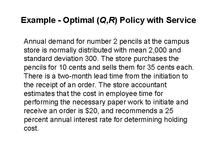
Example - Optimal (Q, R) Policy with Service Annual demand for number 2 pencils at the campus store is normally distributed with mean 2, 000 and standard deviation 300. The store purchases the pencils for 10 cents and sells them for 35 cents each. There is a two-month lead time from the initiation to the receipt of an order. The store accountant estimates that the cost in employee time for performing the necessary paper work to initiate and receive an order is $20, and recommends a 25 percent annual interest rate for determining holding cost.

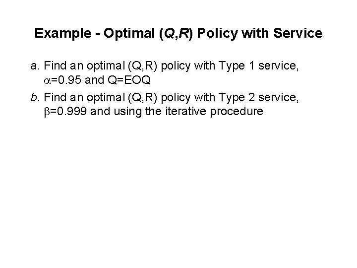
Example - Optimal (Q, R) Policy with Service a. Find an optimal (Q, R) policy with Type 1 service, =0. 95 and Q=EOQ b. Find an optimal (Q, R) policy with Type 2 service, =0. 999 and using the iterative procedure

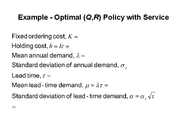
Example - Optimal (Q, R) Policy with Service

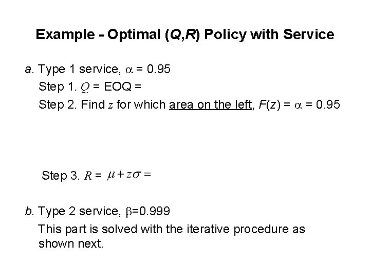
Example - Optimal (Q, R) Policy with Service a. Type 1 service, = 0. 95 Step 1. Q = EOQ = Step 2. Find z for which area on the left, F(z) = = 0. 95 Step 3. R = b. Type 2 service, =0. 999 This part is solved with the iterative procedure as shown next.

Example - Optimal (Q, R) Policy with Service

Example - Optimal (Q, R) Policy with Service

Example - Optimal (Q, R) Policy with Service

Example - Optimal (Q, R) Policy with Service Iteration 2

Example - Optimal (Q, R) Policy with Service

(Q, R) Systems Remark • We solve three versions of the problem of finding an optimal (Q, R) policy – No service constraint – Type 1 service – Type 2 service • All these versions may alternatively and more efficiently solved by Excel Solver. This is discussed during the tutorial.

Multiproduct Systems • Pareto effect – A concept of economics applies to inventory systems – Rank the items in decreasing order of revenue generated – Item group A: top 20% items generate 80% revenue – Item group B: next 30% items generate 15% revenue – Item group A: last 50% items generate 5% revenue

Multiproduct Systems • Exchange curves – Parameters like K and I are not easy to measure – Instead of assigning values to such parameters show the trade off between holding cost and ordering cost for a large number of values of K/I – The effect of changing the ratio K/I is shown by plotting holding cost vs ordering cost – Similarly, instead of assigning a value to type 2 service level , one may show the trade off between cost of safety stock and expected number of stock-outs.

READING AND EXERCISES Lesson 4 Reading: Section 5. 5, pp. 264 -271 (4 th Ed. ), pp. 255 -262 (5 th Ed. ) Section 5. 7 (skim) pp. 275 -280 (4 th Ed. ), pp. 265 -270 (5 th Ed. ) Exercise: 16 and 17, p. 271 (4 th Ed. ), p. 262 (5 th Ed. )