Chapter 12 Independent Demand Inventory Management Types of

Chapter 12 – Independent Demand Inventory Management

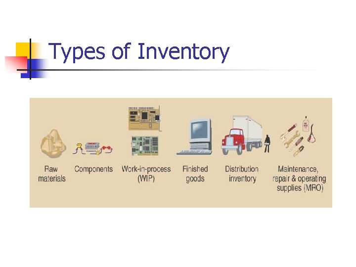
Types of Inventory

Uses of Inventory n n n Anticipation or seasonal inventory Safety stock: buffer demand fluctuations Lot-size or cycle stock: take advantage of quantity discounts or purchasing efficiencies Pipeline or transportation inventory Speculative or hedge inventory protects against some future event, e. g. labor strike Maintenance, repair, and operating (MRO) inventories

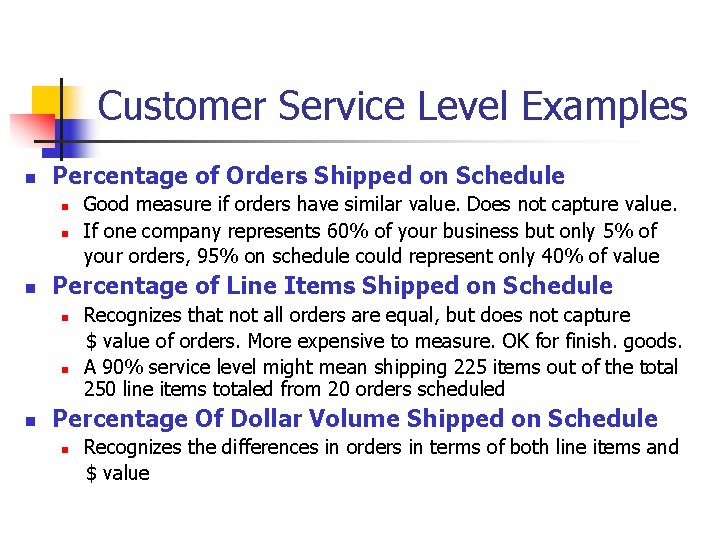
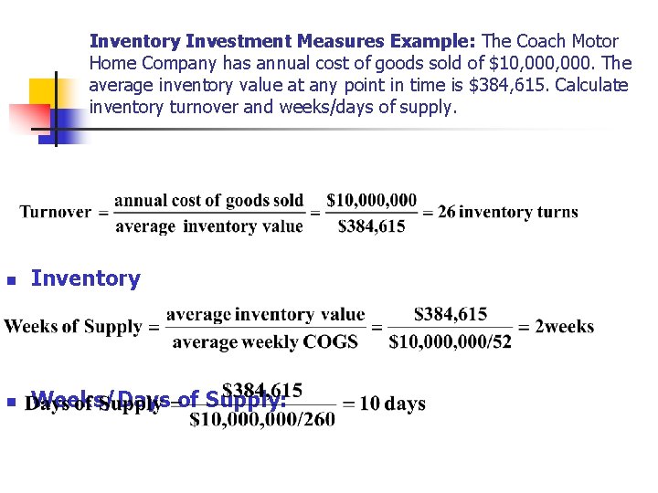
Inventory Management Objectives n Provide desired customer service level: n n n Provide for cost-efficient operations: n n Percentage of orders shipped on schedule Percentage of line items shipped on schedule Percentage of dollar volume shipped on schedule Idle time due to material and component shortages Buffer stock for smooth production flow Maintain a level work force Allowing longer production runs & quantity discounts Minimize inventory related investments: n n Inventory turnover = Annual CGS/Avg Inv ($) Weeks (or days) of supply = Avg Inv ($)/Avg. Wk. Usage

Customer Service Level Examples n Percentage of Orders Shipped on Schedule n n n Percentage of Line Items Shipped on Schedule n n n Good measure if orders have similar value. Does not capture value. If one company represents 60% of your business but only 5% of your orders, 95% on schedule could represent only 40% of value Recognizes that not all orders are equal, but does not capture $ value of orders. More expensive to measure. OK for finish. goods. A 90% service level might mean shipping 225 items out of the total 250 line items totaled from 20 orders scheduled Percentage Of Dollar Volume Shipped on Schedule n Recognizes the differences in orders in terms of both line items and $ value

Inventory Investment Measures Example: The Coach Motor Home Company has annual cost of goods sold of $10, 000. The average inventory value at any point in time is $384, 615. Calculate inventory turnover and weeks/days of supply. n Inventory n Weeks/Days of Supply:

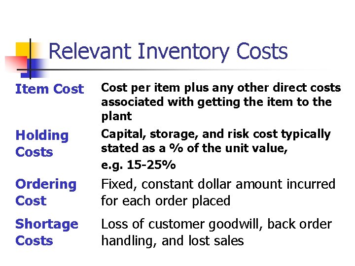
Relevant Inventory Costs Item Cost per item plus any other direct costs associated with getting the item to the plant Holding Costs Capital, storage, and risk cost typically stated as a % of the unit value, e. g. 15 -25% Ordering Cost Fixed, constant dollar amount incurred for each order placed Shortage Costs Loss of customer goodwill, back order handling, and lost sales

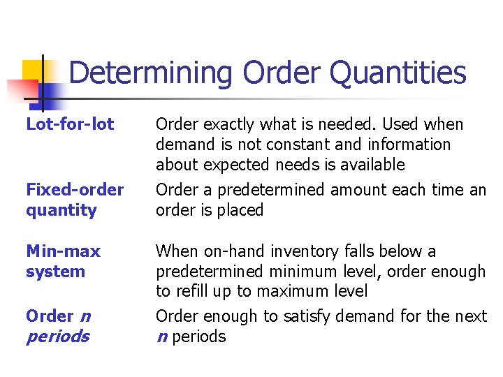
Determining Order Quantities Lot-for-lot Fixed-order quantity Order exactly what is needed. Used when demand is not constant and information about expected needs is available Order a predetermined amount each time an order is placed Min-max system When on-hand inventory falls below a predetermined minimum level, order enough to refill up to maximum level Order n Order enough to satisfy demand for the next n periods

Three Mathematical Models for Determining Order Quantity n Economic Order Quantity (EOQ or Q System) n n n Economic Production Quantity (EPQ) n n A model used to find optimal order q. and RP (Reorder Point) Part of continuous review system which tracks onhand inventory each time a withdrawal is made A model that allows for incremental product delivery Quantity Discount Model n Modifies the EOQ process to consider cases where quantity discounts are available

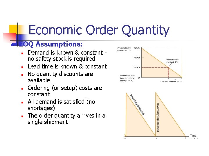
Economic Order Quantity n EOQ Assumptions: n n n Demand is known & constant no safety stock is required Lead time is known & constant No quantity discounts are available Ordering (or setup) costs are constant All demand is satisfied (no shortages) The order quantity arrives in a single shipment

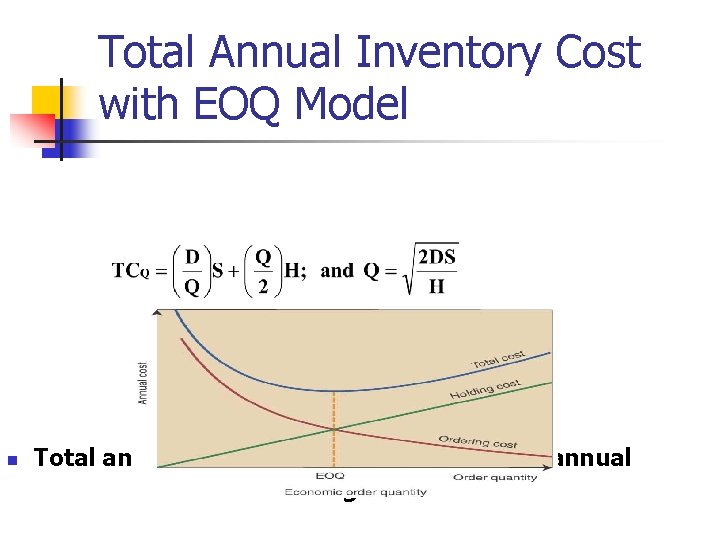
Total Annual Inventory Cost with EOQ Model n Total annual cost= annual ordering cost + annual holding costs

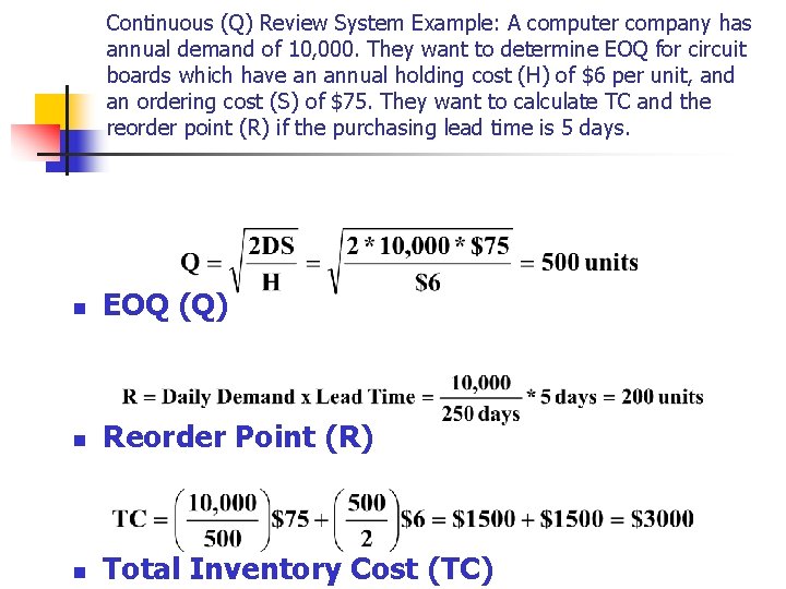
Continuous (Q) Review System Example: A computer company has annual demand of 10, 000. They want to determine EOQ for circuit boards which have an annual holding cost (H) of $6 per unit, and an ordering cost (S) of $75. They want to calculate TC and the reorder point (R) if the purchasing lead time is 5 days. n EOQ (Q) n Reorder Point (R) n Total Inventory Cost (TC)

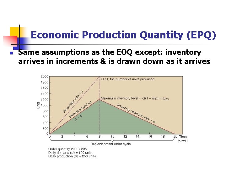
Economic Production Quantity (EPQ) n Same assumptions as the EOQ except: inventory arrives in increments & is drawn down as it arrives

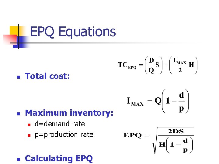
EPQ Equations n Total cost: n Maximum inventory: n n n d=demand rate p=production rate Calculating EPQ

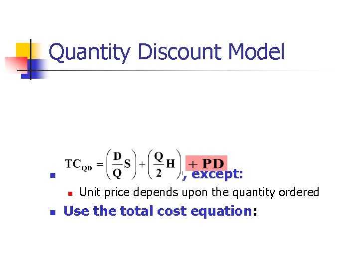
Quantity Discount Model n Same as the EOQ, except: n n Unit price depends upon the quantity ordered Use the total cost equation:

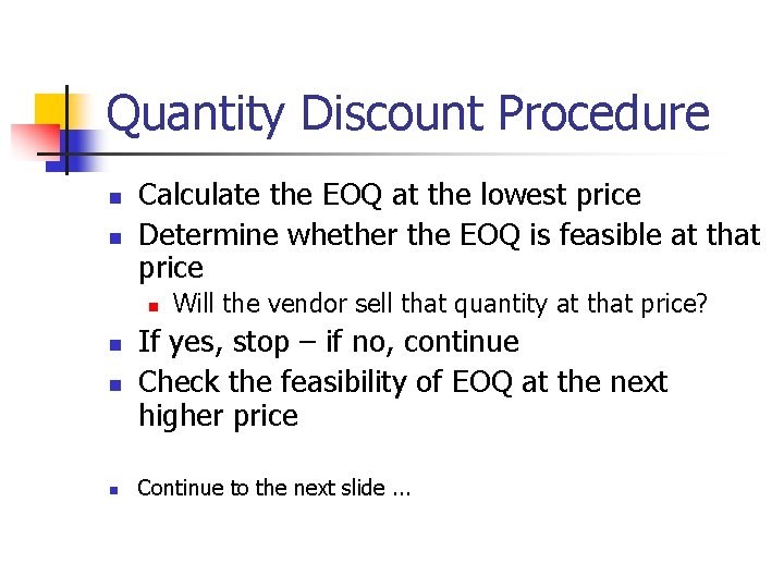
Quantity Discount Procedure n n Calculate the EOQ at the lowest price Determine whether the EOQ is feasible at that price n n Will the vendor sell that quantity at that price? If yes, stop – if no, continue Check the feasibility of EOQ at the next higher price Continue to the next slide. . .

QD Procedure n n n (continued) Continue until you identify a feasible EOQ Calculate the total costs (including total item cost) for the feasible EOQ model Calculate the total costs of buying at the minimum quantity required for each of the cheaper unit prices Compare the total cost of each option & choose the lowest cost alternative Any other issues to consider?

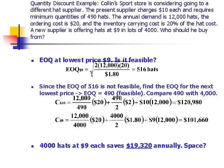
Quantity Discount Example: Collin’s Sport store is considering going to a different hat supplier. The present supplier charges $10 each and requires minimum quantities of 490 hats. The annual demand is 12, 000 hats, the ordering cost is $20, and the inventory carrying cost is 20% of the hat cost. A new supplier is offering hats at $9 in lots of 4000. Who should he buy from? n n n EOQ at lowest price $9. Is it feasible? Since the EOQ of 516 is not feasible, find the EOQ for the next lowest price -> EOQ = 490 (feasible). Compare 490 with 4, 000. 4000 hats at $9 each saves $19, 320 annually. Space?

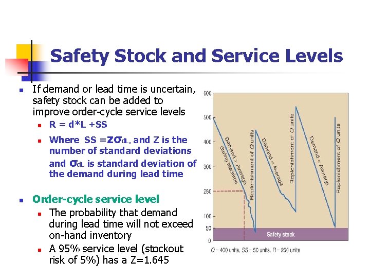
Safety Stock and Service Levels n If demand or lead time is uncertain, safety stock can be added to improve order-cycle service levels n n n R = d*L +SS Where SS =zσd. L, and Z is the number of standard deviations and σd. L is standard deviation of the demand during lead time Order-cycle service level n The probability that demand during lead time will not exceed on-hand inventory n A 95% service level (stockout risk of 5%) has a Z=1. 645

Periodic Review Systems n n Orders are placed at specified, fixed-time intervals (e. g. every Friday), for a order size (Q) to bring onhand inventory (OH) up to the target inventory (TI), similar to the min-max system. Advantages are: n n n No need for a system to continuously monitor item Items ordered from the same supplier can be reviewed on the same day saving purchase order costs Disadvantages: n n n Replenishment quantities (Q) vary Order quantities may not quality for quantity discounts On the average, inventory levels will be higher than Q systems-more stockroom space needed

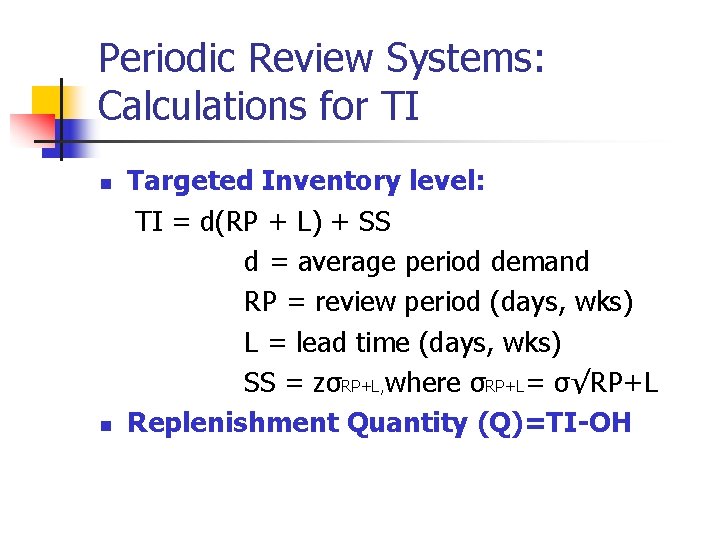
Periodic Review Systems: Calculations for TI n n Targeted Inventory level: TI = d(RP + L) + SS d = average period demand RP = review period (days, wks) L = lead time (days, wks) SS = zσRP+L, where σRP+L= σ√RP+L Replenishment Quantity (Q)=TI-OH

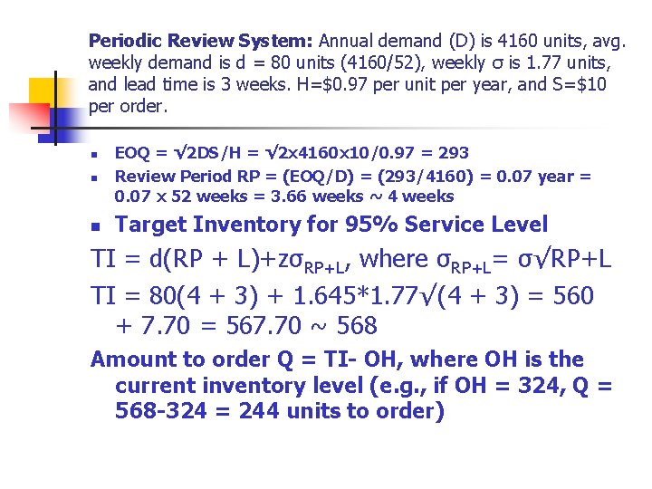
Periodic Review System: Annual demand (D) is 4160 units, avg. weekly demand is d = 80 units (4160/52), weekly σ is 1. 77 units, and lead time is 3 weeks. H=$0. 97 per unit per year, and S=$10 per order. n EOQ = √ 2 DS/H = √ 2 x 4160 x 10/0. 97 = 293 Review Period RP = (EOQ/D) = (293/4160) = 0. 07 year = 0. 07 x 52 weeks = 3. 66 weeks ~ 4 weeks n Target Inventory for 95% Service Level n TI = d(RP + L)+zσRP+L, where σRP+L= σ√RP+L TI = 80(4 + 3) + 1. 645*1. 77√(4 + 3) = 560 + 7. 70 = 567. 70 ~ 568 Amount to order Q = TI- OH, where OH is the current inventory level (e. g. , if OH = 324, Q = 568 -324 = 244 units to order)

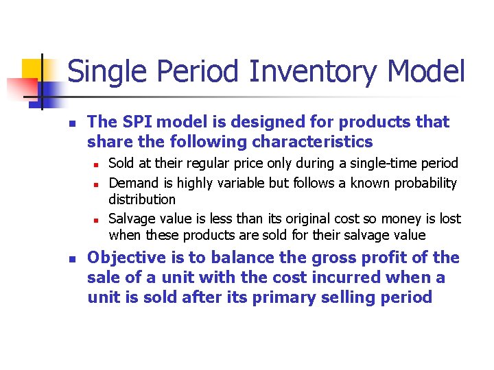
Single Period Inventory Model n The SPI model is designed for products that share the following characteristics n n Sold at their regular price only during a single-time period Demand is highly variable but follows a known probability distribution Salvage value is less than its original cost so money is lost when these products are sold for their salvage value Objective is to balance the gross profit of the sale of a unit with the cost incurred when a unit is sold after its primary selling period

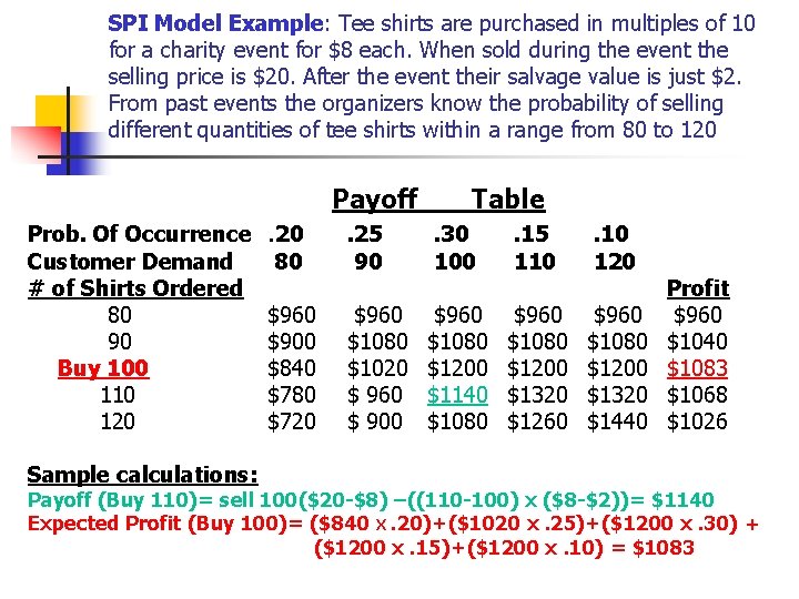
SPI Model Example: Tee shirts are purchased in multiples of 10 for a charity event for $8 each. When sold during the event the selling price is $20. After the event their salvage value is just $2. From past events the organizers know the probability of selling different quantities of tee shirts within a range from 80 to 120 Payoff Prob. Of Occurrence Customer Demand # of Shirts Ordered 80 90 Buy 100 110 120 Sample calculations: . 20 80 $960 $900 $840 $780 $720 Table . 25 90 . 30 100 . 15 110 . 10 120 $960 $1080 $1020 $ 960 $ 900 $960 $1080 $1200 $1140 $1080 $960 $1080 $1200 $1320 $1260 $960 $1080 $1200 $1320 $1440 Profit $960 $1040 $1083 $1068 $1026 Payoff (Buy 110)= sell 100($20 -$8) –((110 -100) x ($8 -$2))= $1140 Expected Profit (Buy 100)= ($840 X. 20)+($1020 x. 25)+($1200 x. 30) + ($1200 x. 15)+($1200 x. 10) = $1083

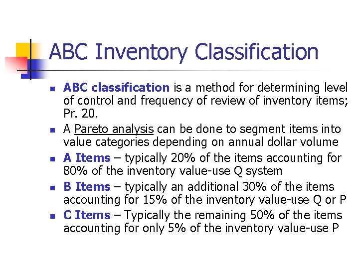
ABC Inventory Classification n n ABC classification is a method for determining level of control and frequency of review of inventory items; Pr. 20. A Pareto analysis can be done to segment items into value categories depending on annual dollar volume A Items – typically 20% of the items accounting for 80% of the inventory value-use Q system B Items – typically an additional 30% of the items accounting for 15% of the inventory value-use Q or P C Items – Typically the remaining 50% of the items accounting for only 5% of the inventory value-use P

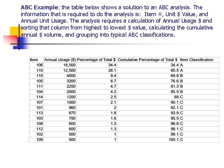
ABC Example: the table below shows a solution to an ABC analysis. The information that is required to do the analysis is: Item #, Unit $ Value, and Annual Unit Usage. The analysis requires a calculation of Annual Usage $ and sorting that column from highest to lowest $ value, calculating the cumulative annual $ volume, and grouping into typical ABC classifications.

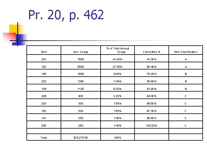
Pr. 20, p. 462 Item Ann. Usage % of Total Annual Usage Cumulative % Item Classification 201 7500 41. 00% A 103 5000 27. 40% 68. 40% A 105 1800 9. 80% 78. 20% B 202 1350 7. 40% 85. 60% B 104 1125 6. 20% 91. 80% B 204 400 2. 20% 94. 00% C 203 300 1. 60% 95. 60% C 102 300 1. 60% 97. 30% C 101 250 1. 40% 98. 60% C 205 250 1. 40% 100. 00% C Total: $18, 275. 00 100%

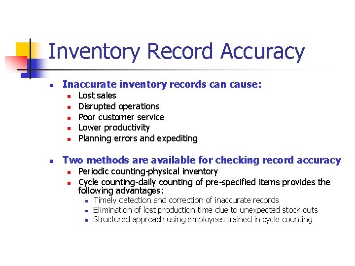
Inventory Record Accuracy n Inaccurate inventory records can cause: n n n Lost sales Disrupted operations Poor customer service Lower productivity Planning errors and expediting Two methods are available for checking record accuracy n n Periodic counting-physical inventory Cycle counting-daily counting of pre-specified items provides the following advantages: n n n Timely detection and correction of inaccurate records Elimination of lost production time due to unexpected stock outs Structured approach using employees trained in cycle counting