Hearty Welcome Probability Theory and Stochastic Process A

Hearty Welcome! Probability Theory and Stochastic Process A Deepika Assistant Professor 1

Course Outcomes • Explain fundamentals of probability theory, random variables and random processes. • Differentiate the mathematical concepts related to probability theory and random processes. • Discuss the characterization of random processes and their properties. • Formulate and solve the engineering problems involving random processes. • Analyze the given probabilistic model of the problem. 2

Probability introduced through sets and relative frequency Experiment: - a random experiment is an to one of several possible outcomes action or process that leads 3

Sample Space • List: “Called the Sample Space” • Outcomes: “Called the Simple Events” • This list must be exhaustive, i. e. ALL possible outcomes included. • Die roll {1, 2, 3, 4, 5} Die roll {1, 2, 3, 4, 5, 6} • • • The list must be mutually exclusive, i. e. no two outcomes can occur at the same time: Die roll {odd number or even number} Die roll{ number less than 4 or even number} 4

Sample Space • A list of exhaustive [don’t leave anything out] and mutually exclusive outcomes [impossible for 2 different events to occur in the same experiment] is called a sample space and is denoted by S. • The outcomes are denoted by O 1, O 2, …, Ok • Using notation from set theory, we can represent the sample space and its outcomes as: • S = {O 1, O 2, …, Ok}

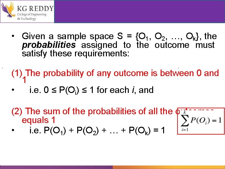
• Given a sample space S = {O 1, O 2, …, Ok}, the probabilities assigned to the outcome must satisfy these requirements: (1) The probability of any outcome is between 0 and 1 • i. e. 0 ≤ P(Oi) ≤ 1 for each i, and (2) The sum of the probabilities of all the outcomes equals 1 • i. e. P(O 1) + P(O 2) + … + P(Ok) = 1

Relative Frequency • Random experiment with sample space S. we shall assign non-negative number called probability to each event in the sample space. • Let A be a particular event in S. then “the probability of event A” is denoted by P(A). • Suppose that the random experiment is repeated n times, if the event A occurs n. A times, then the probability of event A is defined as “Relative frequency “ • Relative Frequency Definition: The probability of an event A is defined as P( A) lim n A n n . 7

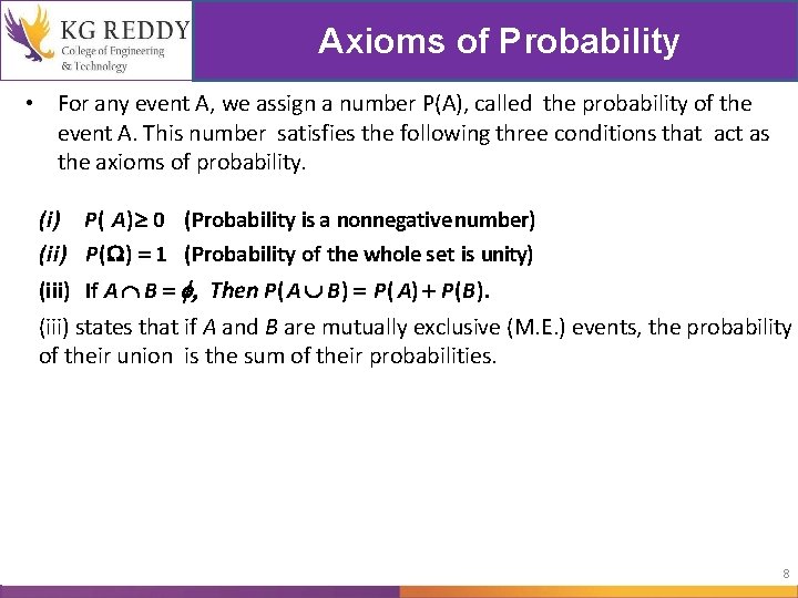
Axioms of Probability • For any event A, we assign a number P(A), called the probability of the event A. This number satisfies the following three conditions that act as the axioms of probability. (i) P( A) 0 (Probability is a nonnegative number) (ii) P( ) 1 (Probability of the whole set is unity) (iii) If A B , Then P( A B) P( A) P(B). (iii) states that if A and B are mutually exclusive (M. E. ) events, the probability of their union is the sum of their probabilities. 8

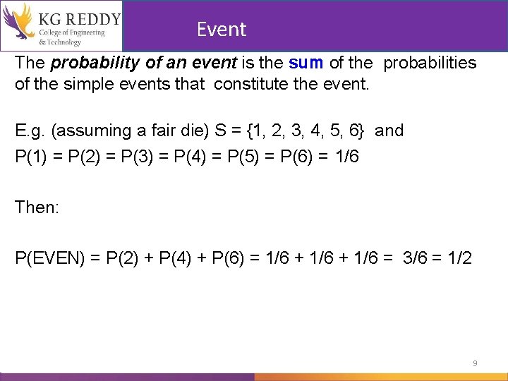
Event The probability of an event is the sum of the probabilities of the simple events that constitute the event. E. g. (assuming a fair die) S = {1, 2, 3, 4, 5, 6} and P(1) = P(2) = P(3) = P(4) = P(5) = P(6) = 1/6 Then: Audit Basics & Types P(EVEN) = P(2) + P(4) + P(6) = 1/6 + 1/6 = 3/6 = 1/2 9

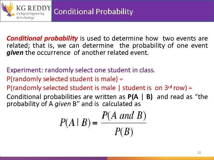
Conditional Probability Conditional probability is used to determine how two events are related; that is, we can determine the probability of one event given the occurrence of another related event. Experiment: randomly select one student in class. P(randomly selected student is male) = Audit Basics & Types P(randomly selected student is male | student is on 3 rd row) = Conditional probabilities are written as P(A | B) and read as “the probability of A given B” and is calculated as 10

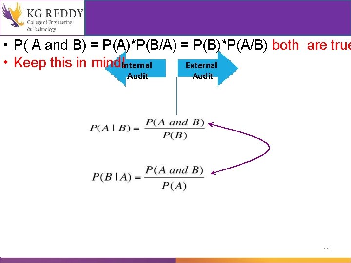
• P( A and B) = P(A)*P(B/A) = P(B)*P(A/B) both are true • Keep this in mind!Internal External Audit 11

Examples on conditional Probability 1. Consider a bag consisting of 100 items of which 80 are non defective and 20 are defective. Suppose that we have to choose 2 items from this lot a) With replacement b) Without replacement. 12

13

14

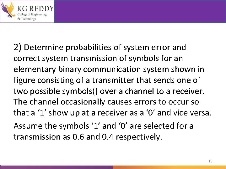
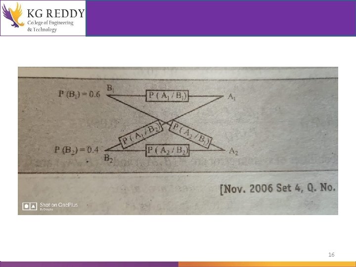
2) Determine probabilities of system error and correct system transmission of symbols for an elementary binary communication system shown in figure consisting of a transmitter that sends one of two possible symbols() over a channel to a receiver. The channel occasionally causes errors to occur so that a ‘ 1’ show up at a receiver as a ‘ 0’ and vice versa. Assume the symbols ‘ 1’ and ‘ 0’ are selected for a transmission as 0. 6 and 0. 4 respectively. 15

16

17

18

19

Bayes’ Law • Bayes’ Law is named for Thomas Bayes, an eighteenth century mathematician. • In its most basic form, if we know P(B | A), • we can apply Bayes’ Law to determine P(A | B) P(B|A) P(A|B) 20

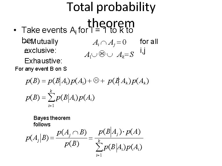
• Total probability theorem Take events A for I = 1 to k to i be: – Mutually Ai Aj 0 exclusive: – Exhaustive: for all i, j A 1 Ak S For any event B on S p(B) p(B A 1) p( A 1) p(B Ak ) p( Ak ) k p(B) p(B Ai ) p( Ai ) i 1 Bayes theorem follows p( Aj B) p( Aj B) p(B Aj ) p( A) k p(B A ) p( A ) i i 1 i

22

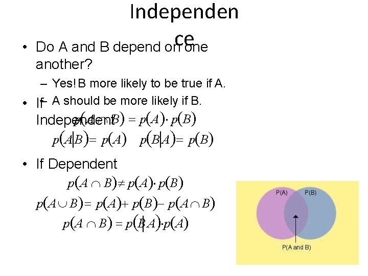
• Independen Do A and B depend once one another? – Yes! B more likely to be true if A. • If– A should be more likely if B. p A B p A p B Independent p A B p A p B A p B • If Dependent p A B p A p B p A B p B A p A

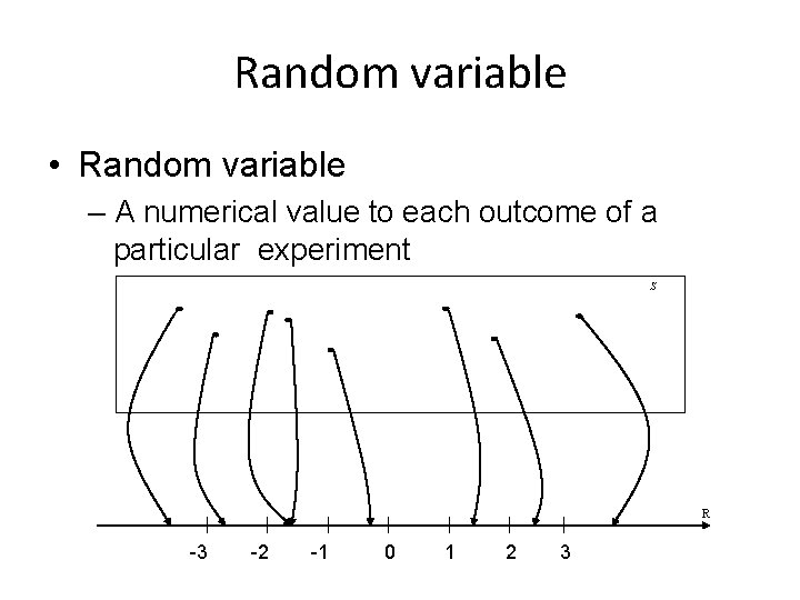
Random variable • Random variable – A numerical value to each outcome of a particular experiment S R -3 -2 -1 0 1 2 3

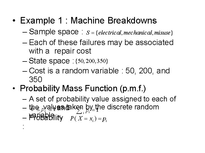
• Example 1 : Machine Breakdowns – Sample space : S {electrical, mechanical, misuse} – Each of these failures may be associated with a repair cost – State space : {50, 200, 350} – Cost is a random variable : 50, 200, and 350 • Probability Mass Function (p. m. f. ) – A set of probability value assigned to each of – the andtaken 0 pvalues 1 discrete random i 1 p i the i by variable xi P( X x ) p – Probability i i :

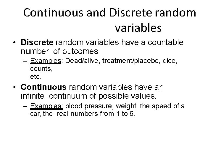
Continuous and Discrete random variables • Discrete random variables have a countable number of outcomes – Examples: Dead/alive, treatment/placebo, dice, counts, etc. • Continuous random variables have an infinite continuum of possible values. – Examples: blood pressure, weight, the speed of a car, the real numbers from 1 to 6.

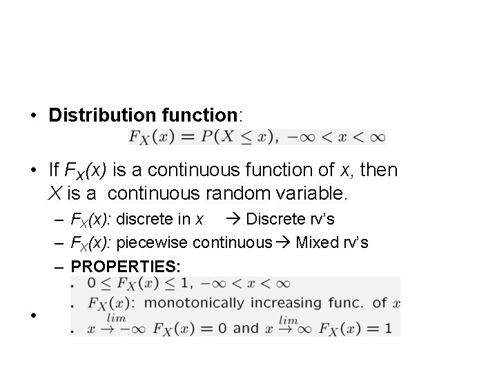
• Distribution function: • If FX(x) is a continuous function of x, then X is a continuous random variable. – FX(x): discrete in x Discrete rv’s – FX(x): piecewise continuous Mixed rv’s – PROPERTIES: •

Probability Density Function (pdf) • X : continuous rv, then, • pdf properties: 1. 2. F (t) t t 0 f (x)dx ,

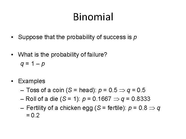
Binomial • Suppose that the probability of success is p • What is the probability of failure? q=1–p • Examples – Toss of a coin (S = head): p = 0. 5 q = 0. 5 – Roll of a die (S = 1): p = 0. 1667 q = 0. 8333 – Fertility of a chicken egg (S = fertile): p = 0. 8 q = 0. 2

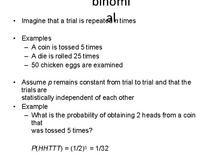
• binomi aln times Imagine that a trial is repeated • Examples – A coin is tossed 5 times – A die is rolled 25 times – 50 chicken eggs are examined • Assume p remains constant from trial to trial and that the trials are statistically independent of each other • Example – What is the probability of obtaining 2 heads from a coin that was tossed 5 times? P(HHTTT) = (1/2)5 = 1/32

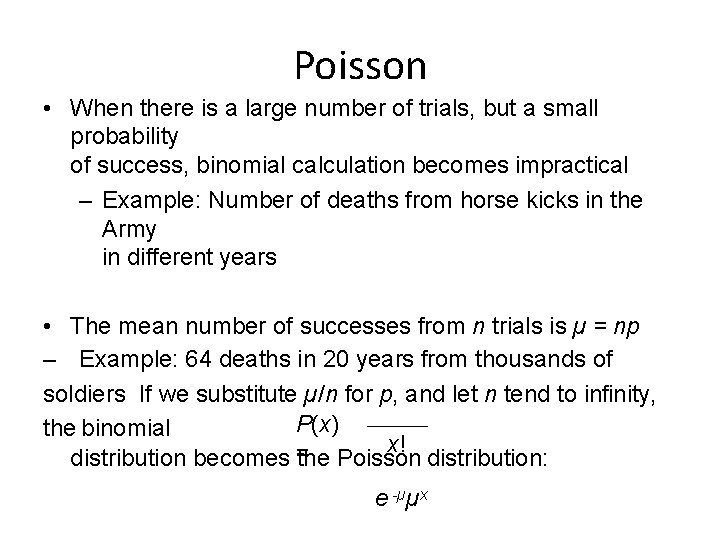
Poisson • When there is a large number of trials, but a small probability of success, binomial calculation becomes impractical – Example: Number of deaths from horse kicks in the Army in different years • The mean number of successes from n trials is µ = np – Example: 64 deaths in 20 years from thousands of soldiers If we substitute µ/n for p, and let n tend to infinity, P(x) the binomial x! = distribution becomes the Poisson distribution: e -µµx

poisson • Poisson distribution is applied where random events in space or time are expected to occur • Deviation from Poisson distribution may indicate some degree of nonrandomness in the events under study • Investigation of cause may be of interest

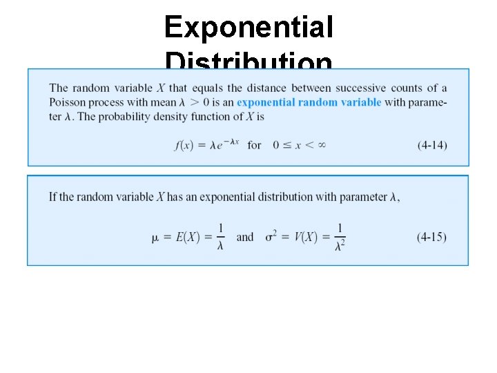
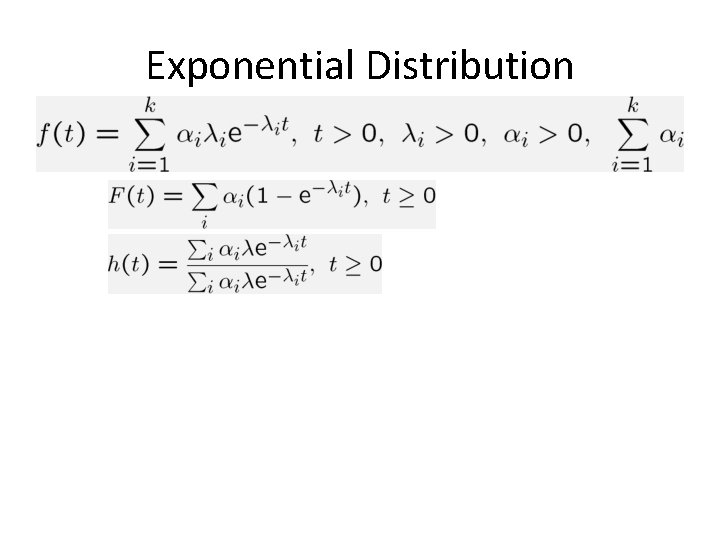
Exponential Distribution

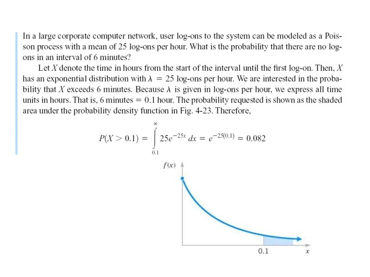
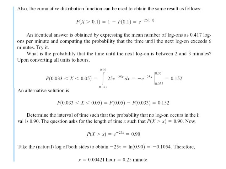
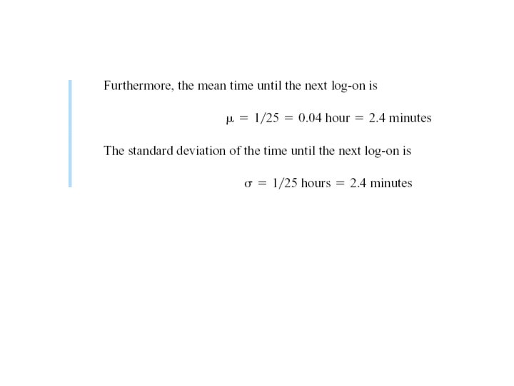
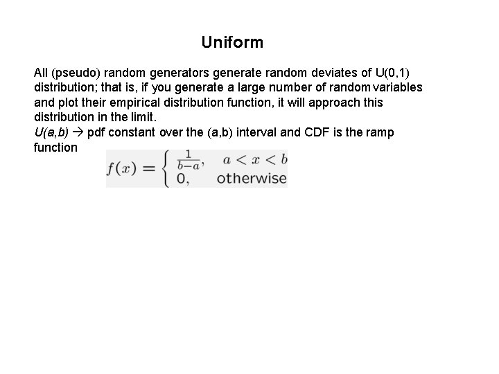
Uniform All (pseudo) random generators generate random deviates of U(0, 1) distribution; that is, if you generate a large number of random variables and plot their empirical distribution function, it will approach this distribution in the limit. U(a, b) pdf constant over the (a, b) interval and CDF is the ramp function

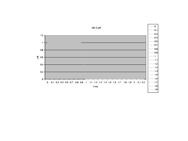
0 U(0, 1) pdf 0. 1 0. 2 1. 2 0. 3 0. 6 1 0. 7 0. 8 cdf 0. 9 1 0. 6 1. 1 1. 2 0. 4 1. 3 1. 4 0. 2 1. 5 1. 6 0 0 0. 1 0. 2 0. 3 0. 6 0. 7 0. 8 0. 9 1 1. 2 1. 3 1. 4 1. 5 1. 6 1. 7 time 1. 8 1. 9 2 2. 1 2. 2 1. 7 1. 8 1. 9

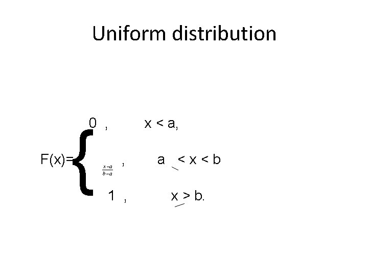
Uniform distribution 0 , { F(x)= x a b a x < a, , 1 , a <x<b x > b.

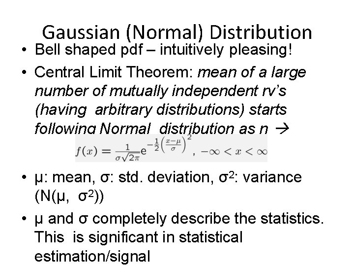
Gaussian (Normal) Distribution • Bell shaped pdf – intuitively pleasing! • Central Limit Theorem: mean of a large number of mutually independent rv’s (having arbitrary distributions) starts following Normal distribution as n • μ: mean, σ: std. deviation, σ2: variance (N(μ, σ2)) • μ and σ completely describe the statistics. This is significant in statistical estimation/signal

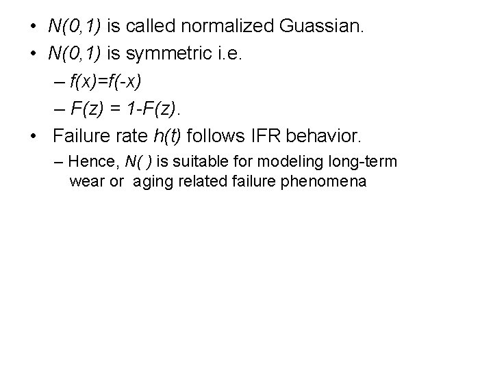
• N(0, 1) is called normalized Guassian. • N(0, 1) is symmetric i. e. – f(x)=f(-x) – F(z) = 1 -F(z). • Failure rate h(t) follows IFR behavior. – Hence, N( ) is suitable for modeling long-term wear or aging related failure phenomena

Exponential Distribution

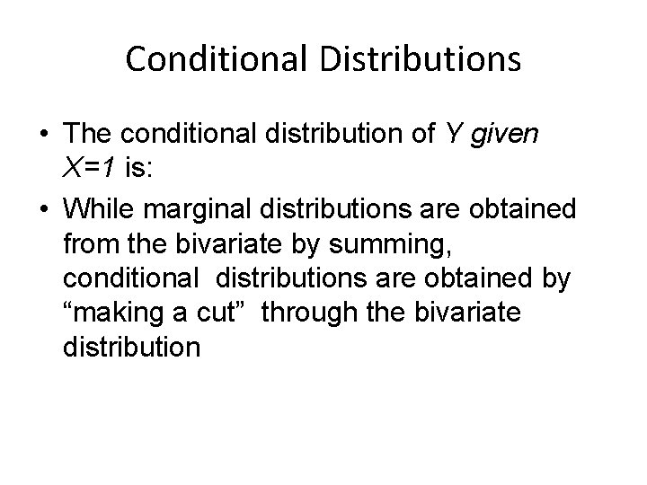
Conditional Distributions • The conditional distribution of Y given X=1 is: • While marginal distributions are obtained from the bivariate by summing, conditional distributions are obtained by “making a cut” through the bivariate distribution

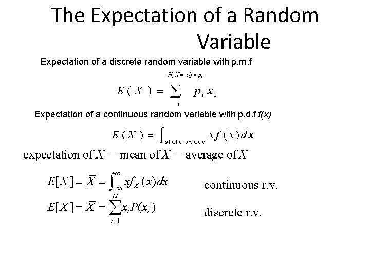
The Expectation of a Random Variable Expectation of a discrete random variable with p. m. f P( X xi ) pi E( X ) pi xi i Expectation of a continuous random variable with p. d. f f(x) E(X ) state s p ace xf ( x)dx expectation of X = mean of X = average of X E[ X ] X xf X (x)dx continuous r. v. E[ X ] X xi P(xi ) discrete r. v. N i 1

f X (x a) f X ( x a), x E[ X ] a X r. v. Y =g( X ) r. v. Ex: Y g( X ) X 2 1 P( X 0) P( X 1) 3 P(Y 0) Expectation 1 3 expectation of a function of a r. v. X E[g( X )] g(x) f X (x)dx continuous r. v. E[g( X )] g(x i )P(xi ) discrete r. v. N i 1 conditional expectation of a r. v. X E[ X B] xf X (x B)dx continuous r. v. E[ X B] xi P(xi B) discrete r. v. N i 1 P(Y 1) 2 3

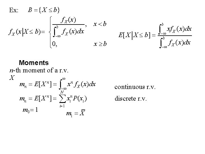
Ex: B {X b} f X (x) , x b b f X (x X b) f X (x)dx x b 0, Moments n-th moment of a r. v. X n mn E[ X ] xn f X (x)dx N mn E[ X n ] xin P(xi ) m 0 1 i 1 m 1 X b E[ X X b] b continuous r. v. discrete r. v. xf X (x)dx

properties of expectation: (1) E[c] c c -- constant (2) E[ag( X ) bh( X )] a. E[g( X )] b. E[h( X )] PF: E[c] cf X (x)dx c E[ag( X ) bh( X )] {ag(x) bh(x)} f X (x)dx a g(x) f X (x)dx b h(x) f X (x)dx a. E[g(X )] b. E[h(X )]

variance of a r. v. X X 2 2 E[( X X )2 ] E[ X 2 2 XX X 2 ] E[ X 2 ] 2 XE[ X ] X 2 m m 2 2 1 standard deviation of a r. v. X X ( 0) skewness of a r. v. X Ex 3. 2 -1 & Ex 3. 22: exponential r. v. 3 X 3 f X (x) symmetric about x X 1 x a e b , x a f X (x) b 0, x a 3 0

1 x a m 1 E[ X ] x e b dx a b a b 1 x a m 2 E[ X 2 ] x 2 e b dx (a b)2 b 2 a b 2 m m 2 b 2 X 2 2 1 x a 1 m 3 E[ X 3 ] x 3 e b dx a 3 3 a 2 b 6 ab 2 6 b 3 a b 2 3 3 E[( X X )3 ] E[ X 3 3 X 2 X 3 XX 2 X 3 ] m 3 3 m 1 m 2 3 m 1 a 3 3 a 2 b 6 ab 2 6 b 3 3(a b){(a b)2 b 2 } 2(a b)3 2 b 3 3 2 b skewness of a r. v. X � 33 2 3 X b

X Chebychev's inequality P[ X X ] 2 2 (x X ) f. X (x)dx x X (x X )2 f. X (x)dx 2 X 2 2 Markov's inequality x X f (x)dx 2 P[ X X ] X P[ X 0] 0 P[ X a] E[X ] 2 a 1 Ex 3. 2 -3: P[ X X 3 X ] �X 2 9 X 9

Characteristic function of r. v. X X ( ) E[e j X ] f X (x)e j x dx 1 f X (x) 2 X ( ) X d n ( ) 0 X ( )e f X (x) e j x n Fourier transform d dx n f X (x) j x e n d X ( ) n mn ( j) d n 0 j x dx f X (x)dx 1 X (0) 0 j n f X (x)x ndx j n E[ X n ]

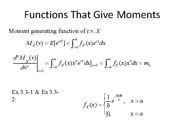
Functions That Give Moments Moment generating function of r. v. X M X (v) E[e ] v. X d n M (v) X n dv v 0 f X (x)evx dx n vx f X (x)x e dx Ex 3. 3 -1 & Ex 3. 32: v 0 f X (x)x ndx mn 1 x a e b , x a f X (x) b 0, x a

X ( ) E[e a j X 1 ] e b ( 1 j ) a b a j a e e 1 b e e b ( 1 j ) 1 j b b va e M X (v) E[ev. X ] 1 vb 1 ( j ) x b a b 1 e dx e b ( 1 j ) b d X ( ) d a b 0 x a d X ( ) jae j a (1 j b) e j a jb (1 j b)2 d d. M X (v) aeva (1 vb) e va b dv m 1 ( j) ( 1 j ) x b (1 vb)2 d. M (v) m 1 �X a b dv v 0

Ex 3. 3 -3: Chernoff's inequality v 0 P[ X a] a f X (x)dx f X (x)u(x a)dx f X (x)e v( x a ) dx e va M X (v) Transformations of a Random Variable

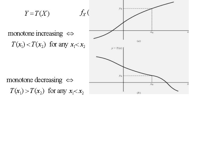
Y T(X ) f. X (x) given f. Y (y) ? monotone increasing T (x 1) T (x 2 ) for any x 1 x 2 monotone decreasing T (x 1) T (x 2 ) for any x 1 x 2

Assume monotone increasing T ( ) FY( y 0 ) P[Y y 0 ] P[ X x 0 ] FX (x 0 ) y 0 f. Y ( y)dy T 1 ( y 0 ) f X (x)dx 1 d. T ( y 0 ) f. Y ( y 0 ) f X [T 1 ( y 0 )] dy 0 d. T 1( y) dx f. Y ( y) f X [T ( y)] f X (x) dy dy 1 Y T (X )

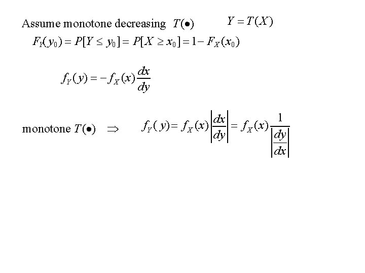
Y T (X ) Assume monotone decreasing T ( ) FY( y 0 ) P[Y y 0 ] P[ X x 0 ] 1 FX (x 0 ) f. Y ( y) f X (x) monotone T ( ) dx dy f. Y ( y) f X (x) 1 dx f X (x) dy dy dx

nonmonotone T ( ) Y T(X ) f. Y ( y) n f. X (xn ) d. T (x) dx x xn

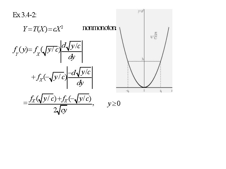
Ex 3. 4 -2: Y T(X ) c. X 2 nonmonotone d y /c f ( y) f ( y / c) Y X dy d y /c f X ( y / c) dy f. X ( y / c) 2 cy , y 0

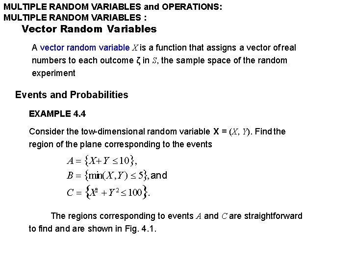
MULTIPLE RANDOM VARIABLES and OPERATIONS: MULTIPLE RANDOM VARIABLES : Vector Random Variables A vector random variable X is a function that assigns a vector of real numbers to each outcome ζ in S, the sample space of the random experiment Events and Probabilities EXAMPLE 4. 4 Consider the tow-dimensional random variable X = (X, Y). Find the region of the plane corresponding to the events A X Y 10 , B min( X , Y ) 5 , and C X 2 Y 2 100. The regions corresponding to events A and C are straightforward to find are shown in Fig. 4. 1.

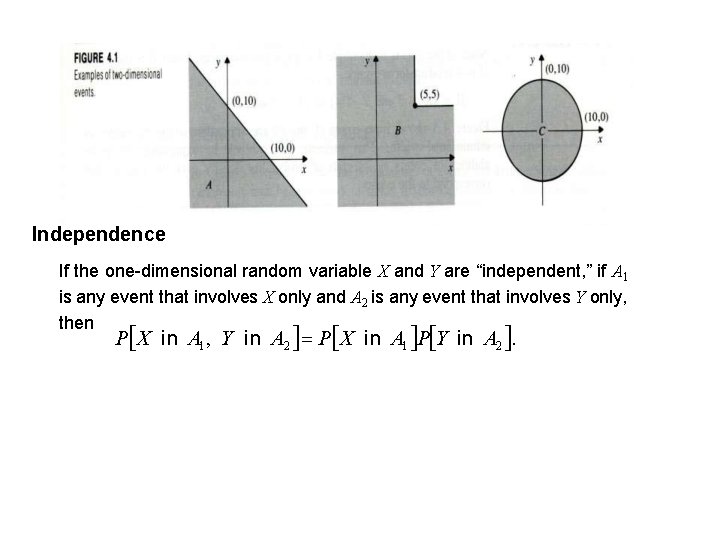
Independence If the one-dimensional random variable X and Y are “independent, ” if A 1 is any event that involves X only and A 2 is any event that involves Y only, then P X in A 1 , Y in A 2 P X in A 1 P Y in A 2 .

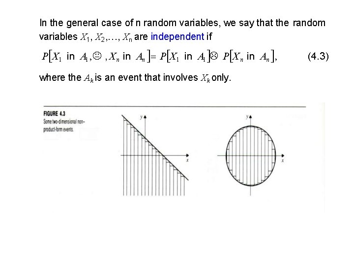
In the general case of n random variables, we say that the random variables X 1, X 2, …, Xn are independent if P X 1 in A 1 , , X n in An P X 1 in A 1 P X n in An , where the Ak is an event that involves Xk only. (4. 3)

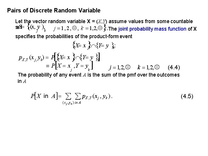
Pairs of Discrete Random Variable Let the vector random variable X = (X, Y) assume values from some countable se. St (x, y ), j 1, 2, , k 1, 2, . The joint probability mass function of X j k specifies the probabilities of the product-form event X x Y y : y ) P X x Y y j p X , Y (x j, k j P X x , Y y j k k k j 1, 2, k 1, 2, (4. 4) The probability of any event A is the sum of the pmf over the outcomes in A P X in A p ( x j , yk ) in A X , Y (x j , yk ). (4. 5)

p (x , yk ) 1. (4. 6) X , Y j j 1 k 1 The marginal probability mass functions : p X (x j ) P X x j P X x , Y anything j P X x and Y y X x j p. X, Y (x j , yk ) , 1 j and Y y 2 (4. 7 a) k 1 p. Y ( yk ) P Y yk p. X, Y ( x j , yk ). j 1 (4. 7 b)

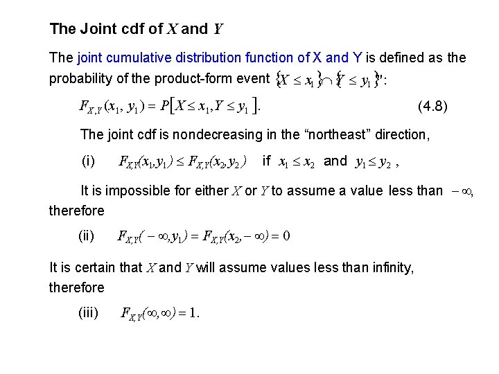
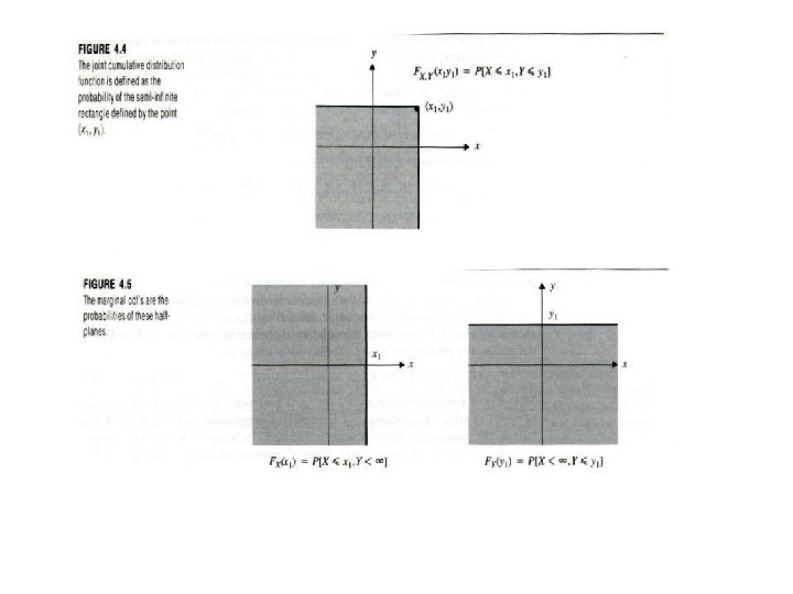
The Joint cdf of X and Y The joint cumulative distribution function of X and Y is defined as the probability of the product-form event X x 1 Y y 1 ": FX , Y (x 1 , y 1 ) P X x 1 , Y y 1 . (4. 8) The joint cdf is nondecreasing in the “northeast” direction, (i) FX, Y(x 1, y 1 ) FX, Y(x 2, y 2 ) if x 1 x 2 and y 1 y 2 , It is impossible for either X or Y to assume a value less than , therefore (ii) FX, Y( , y 1 ) FX, Y(x 2, ) 0 It is certain that X and Y will assume values less than infinity, therefore (iii) FX, Y( , ) 1.

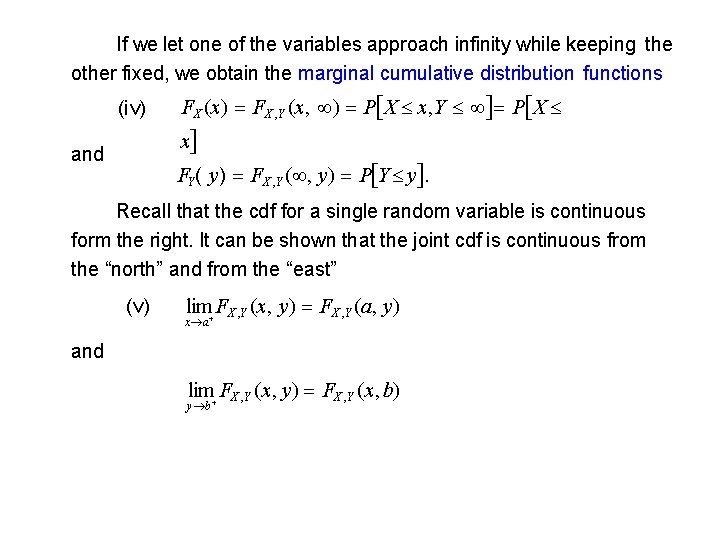
If we let one of the variables approach infinity while keeping the other fixed, we obtain the marginal cumulative distribution functions (iv) FX (x) FX , Y (x, ) P X x, Y P X x and FY( y) FX , Y ( , y) P Y y. Recall that the cdf for a single random variable is continuous form the right. It can be shown that the joint cdf is continuous from the “north” and from the “east” (v) lim FX , Y (x, y) FX , Y (a, y) x a and lim FX , Y (x, y) FX , Y (x, b) y b

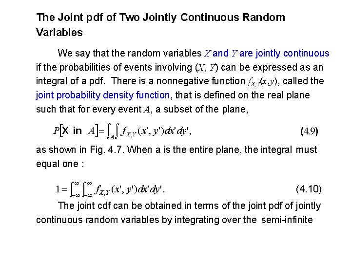
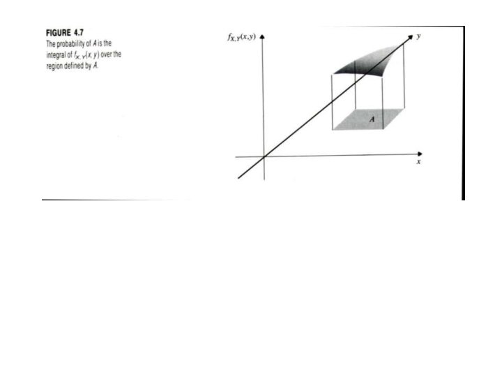
The Joint pdf of Two Jointly Continuous Random Variables We say that the random variables X and Y are jointly continuous if the probabilities of events involving (X, Y) can be expressed as an integral of a pdf. There is a nonnegative function f. X, Y(x, y), called the joint probability density function, that is defined on the real plane such that for every event A, a subset of the plane, P X in A A f X , Y (x', y')dx' dy', (4. 9) as shown in Fig. 4. 7. When a is the entire plane, the integral must equal one : 1 f X , Y (x', y')dx' dy'. (4. 10) The joint cdf can be obtained in terms of the joint pdf of jointly continuous random variables by integrating over the semi-infinite

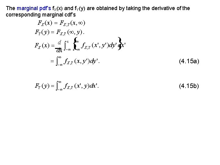
The marginal pdf’s f. X(x) and f. Y(y) are obtained by taking the derivative of the corresponding marginal cdf’s FX (x) FX , Y (x, ) FY ( y) FX , Y ( , y). d x FX (x) dx f X , Y f X , Y (x, y')dy'. (x', y')dy' dx' FY ( y) f X , Y (x', y)dx'. (4. 15 a) (4. 15 b)

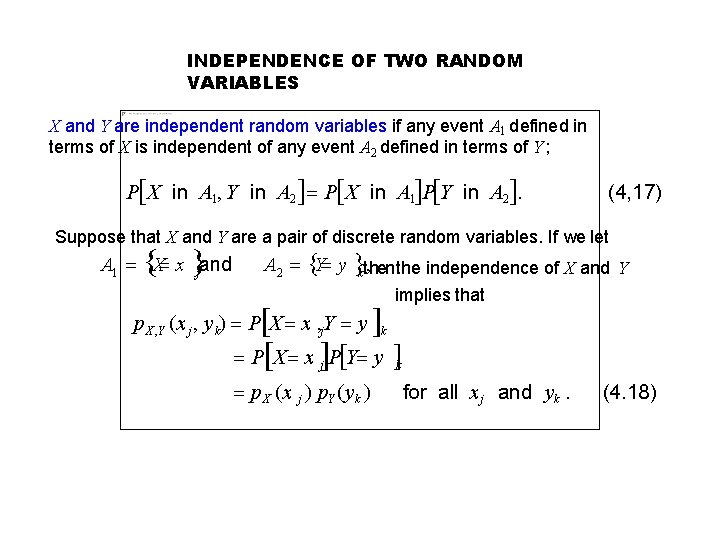
INDEPENDENCE OF TWO RANDOM VARIABLES X and Y are independent random variables if any event A 1 defined in terms of X is independent of any event A 2 defined in terms of Y ; P X in A 1, Y in A 2 P X in A 1 P Y in A 2. (4, 17) Suppose that X and Y are a pair of discrete random variables. If we let A 1 X x jand A 2 Y y kt, hen the independence of X and Y p X , Y (x j , y k) P X x , Y j y k P X x j P Y y p X (x j ) p. Y ( yk ) implies that k for all x j and yk. (4. 18)

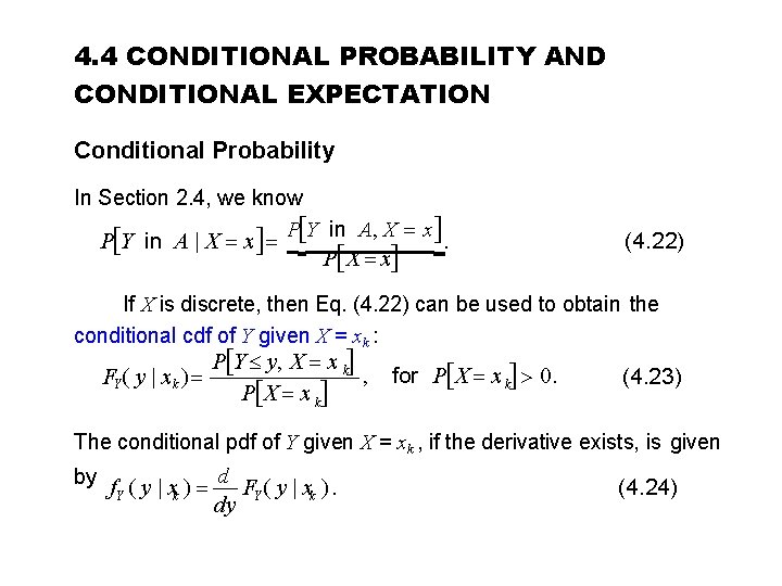
4. 4 CONDITIONAL PROBABILITY AND CONDITIONAL EXPECTATION Conditional Probability In Section 2. 4, we know P Y in A, X x P Y in A | X x P X x . (4. 22) If X is discrete, then Eq. (4. 22) can be used to obtain the conditional cdf of Y given X = xk : FY( y | xk ) P Y y, X x k , P X x k for P X x k 0. (4. 23) The conditional pdf of Y given X = xk , if the derivative exists, is given by f. Y ( y | xk ) d FY ( y | xk ). dy (4. 24)

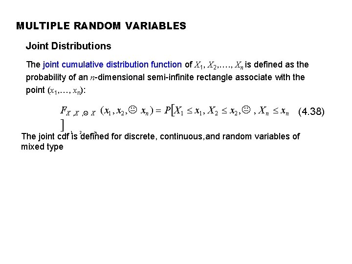
MULTIPLE RANDOM VARIABLES Joint Distributions The joint cumulative distribution function of X 1, X 2, …. , Xn is defined as the probability of an n-dimensional semi-infinite rectangle associate with the point (x 1, …, xn): FX . , X , X 1 2 n (x 1 , x 2 , xn ) P X 1 x 1 , X 2 x 2 , , X n xn (4. 38) The joint cdf is defined for discrete, continuous, and random variables of mixed type

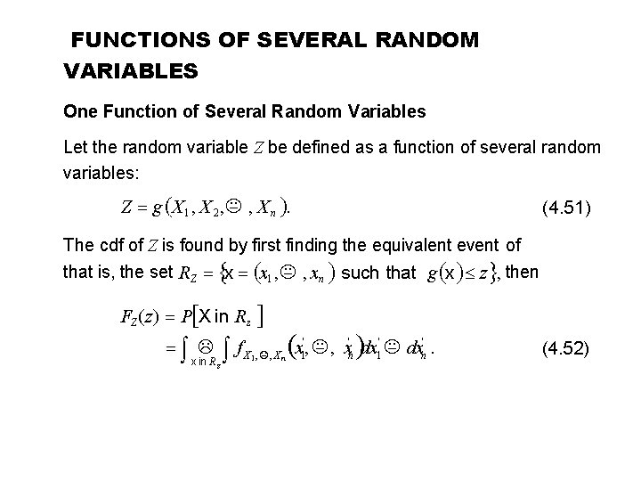
FUNCTIONS OF SEVERAL RANDOM VARIABLES One Function of Several Random Variables Let the random variable Z be defined as a function of several random variables: Z g X 1 , X 2 , , X n . (4. 51) The cdf of Z is found by first finding the equivalent event of that is, the set RZ x x 1 , , xn such that g x z , then FZ (z) P X in Rz x in R z f X 1 , , X n x 1', , xn' dx 1' dxn'. (4. 52)

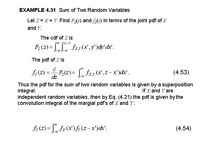
EXAMPLE 4. 31 Sum of Two Random Variables Let Z = X + Y. Find FZ(z) and f. Z(z) in terms of the joint pdf of X and Y. The cdf of Z is z x' FZ (z) f X , Y (x', y')dy' dx'. The pdf of Z is d f Z (z) FZ(z) dz f X , Y (x', z x')dx'. (4. 53) Thus the pdf for the sum of two random variables is given by a superposition integral. If X and Y are independent random variables, then by Eq. (4. 21) the pdf is given by the convolution integral of the margial pdf’s of X and Y : f Z (z) f X (x') f. Y (z x')dx'. (4. 54)

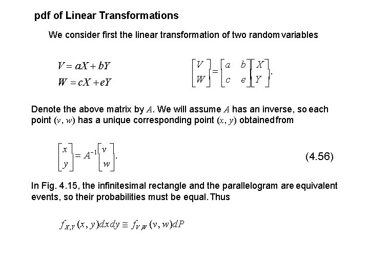
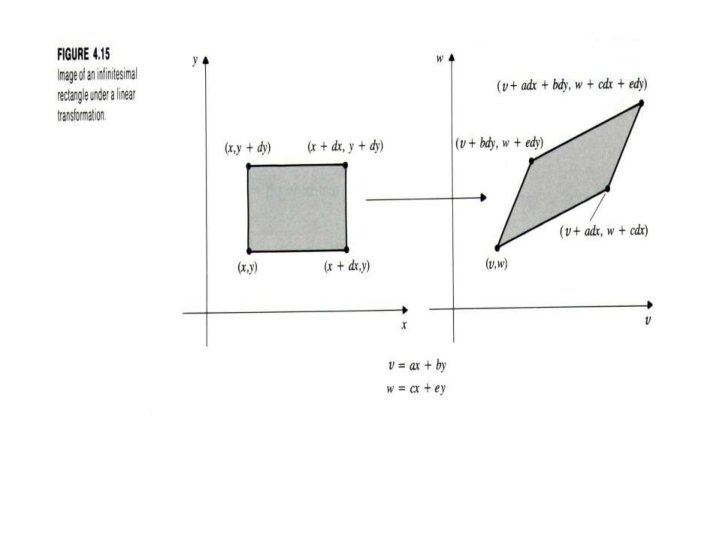
pdf of Linear Transformations We consider first the linear transformation of two random variables V a. X b. Y W c. X e. Y V a b X W c e Y . Denote the above matrix by A. We will assume A has an inverse, so each point (v, w) has a unique corresponding point (x, y) obtained from x 1 v A y w . (4. 56) In Fig. 4. 15, the infinitesimal rectangle and the parallelogram are equivalent events, so their probabilities must be equal. Thus f X , Y (x, y)dxdy f. V , W (v, w)d. P

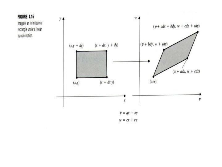
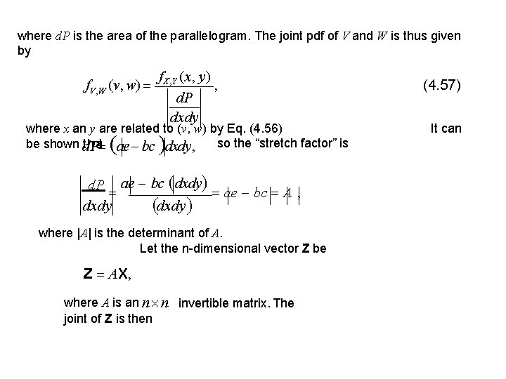
where d. P is the area of the parallelogram. The joint pdf of V and W is thus given by f. X , Y (x, y) f. V , W (v, w) , d. P dxdy where x an y are related to (v, w) by Eq. (4. 56) so the “stretch factor” is be shown d t h. Pa t ae bc dxdy , d. P ae bc dxdy ae bc A , dxdy where |A| is the determinant of A. Let the n-dimensional vector Z be Z AX, where A is an n n invertible matrix. The joint of Z is then (4. 57) It can

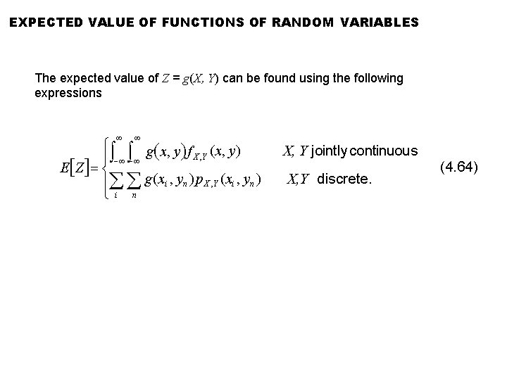
EXPECTED VALUE OF FUNCTIONS OF RANDOM VARIABLES The expected value of Z = g(X, Y) can be found using the following expressions (x, y) g x, y f X , Y E Z g(x i , yn ) p. X , Y (xi , yn ) i n X, Y jointly continuous X, Y discrete. (4. 64)

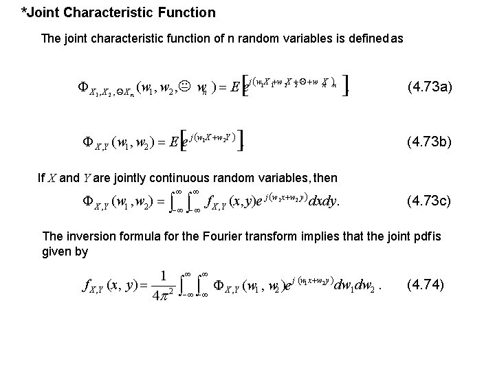
*Joint Characteristic Function The joint characteristic function of n random variables is defined as X 1 , X 2 , X n (w 1 , w 2 , wn ) E ej w 1 X 1 w 2 X 2 w Xn n . X , Y (w 1 , w 2 ) E e j w 1 X w 2 Y . (4. 73 a) (4. 73 b) If X and Y are jointly continuous random variables, then X , Y (w 1 , w 2) f X , Y (x, y)e j w 1 x w 2 y dxdy. (4. 73 c) The inversion formula for the Fourier transform implies that the joint pdf is given by f X , Y (x, y) 1 4 2 X , Y (w 1 , w 2 )e j w 1 x w 2 y dw 1 dw 2. (4. 74)

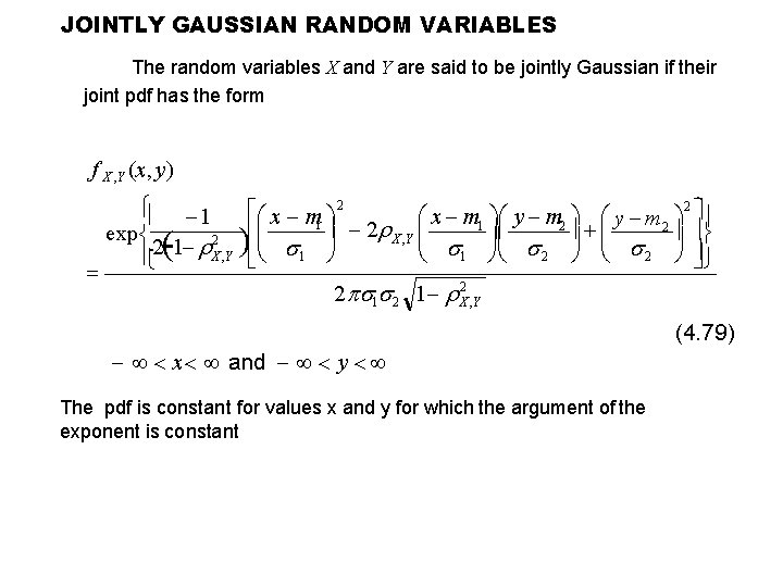
JOINTLY GAUSSIAN RANDOM VARIABLES The random variables X and Y are said to be jointly Gaussian if their joint pdf has the form f X , Y (x, y) 2 1 x m 2 x m y m 1 1 2 2 2 X , Y exp 2 1 2 2 1 X , Y 1 2 1 X 2 , Y (4. 79) x and y The pdf is constant for values x and y for which the argument of the exponent is constant

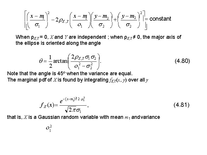
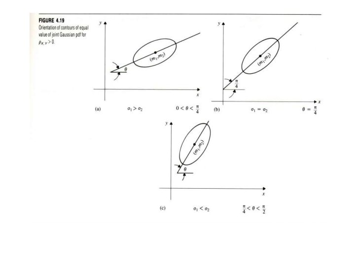
2 x m 2 x m y m 2 1 1 2 constant 2 X , Y 1 1 2 2 When ρX, Y = 0, X and Y are independent ; when ρX, Y ≠ 0, the major axis of the ellipse is oriented along the angle 2 1 arctan X 2 , Y 1 2 2 1 2 (4. 80) Note that the angle is 45º when the variance are equal. The marginal pdf of X is found by integrating f. X, Y(x, y) over all y f X (x) e x m 1 2/ 2 12 2 1 , that is, X is a Gaussian random variable with mean m 1 and variance 12 (4. 81)

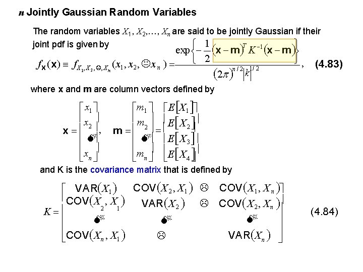
n Jointly Gaussian Random Variables The random variables X 1, X 2, …, Xn are said to be jointly Gaussian if their joint pdf is given by T 1 1 exp x m K x m , 2 f X (x) f X 1, X 2 , , X n (x 1 , x 2 , x n ) 2 n / 2 k 1/ 2 (4. 83) where x and m are column vectors defined by x 1 x 2 x , x n m 1 E X 1 m E X 2 m 2 E X 3 m E X n 4 and K is the covariance matrix that is defined by COV X 2 , X 1 COV X 1 , X n VAR X 1 COV X , X VAR X COV X , X 2 2 n 2 1 K VAR X n COV X n , X 1 (4. 84)

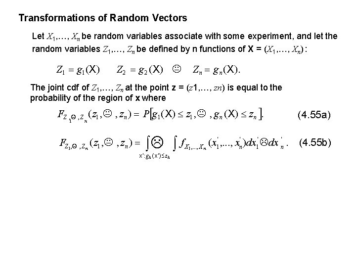
Transformations of Random Vectors Let X 1, …, Xn be random variables associate with some experiment, and let the random variables Z 1, …, Zn be defined by n functions of X = (X 1, …, Xn) : Z 1 g 1(X) Z 2 g 2 (X) Z n g n (X). The joint cdf of Z 1, …, Zn at the point z = (z 1, …, zn) is equal to the probability of the region of x where FZ , , Z (z 1 , , z n ) P g 1 (X) z 1 , , g n (X) z n . 1 n FZ 1 , , Z n (z 1 , , zn ) f x': gk ( x') z k (4. 55 a) ' ' (x , . . . , x )dx dx (4. 55 b) X 1 , . . . , X n 1 n.

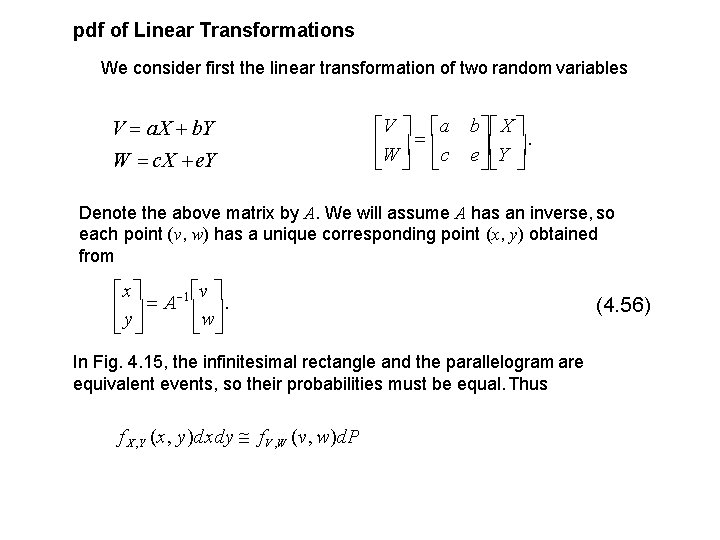
pdf of Linear Transformations We consider first the linear transformation of two random variables V a. X b. Y W c. X e. Y V a b X W c e Y . Denote the above matrix by A. We will assume A has an inverse, so each point (v, w) has a unique corresponding point (x, y) obtained from x 1 v A y w . In Fig. 4. 15, the infinitesimal rectangle and the parallelogram are equivalent events, so their probabilities must be equal. Thus f X , Y (x, y)dxdy f. V , W (v, w)d. P (4. 56)

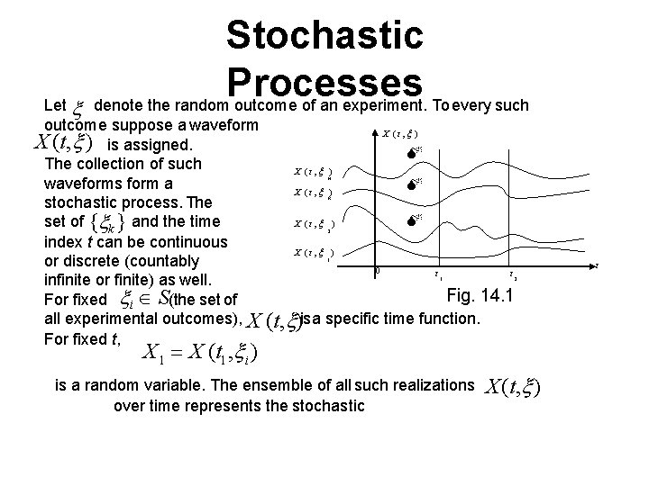
Stochastic Processes Let denote the random outcome of an experiment. To every such outcome suppose a waveform X (t, ) is assigned. The collection of such waveforms form a stochastic process. The set of { k } and the time index t can be continuous or discrete (countably infinite or finite) as well. For fixed i S(the set of all experimental outcomes), X For fixed t, X (t , ) n X (t , ) k 2 X (t , ) 1 0 t t 1 t 2 Fig. 14. 1 (t, )is a specific time function. X 1 X (t 1 , i ) is a random variable. The ensemble of all such realizations over time represents the stochastic X (t, )

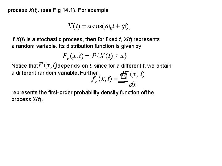
process X(t). (see Fig 14. 1). For example X (t) a cos( 0 t ), If X(t) is a stochastic process, then for fixed t, X(t) represents a random variable. Its distribution function is given by FX (x, t) P{X (t) x} Notice that. F (x, t) X depends on t, since for a different t, we obtain a different random variable. Further d. F (x, t) f X (x, t) �X dx represents the first-order probability density function of the process X(t).

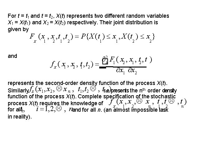
For t = t 1 and t = t 2, X(t) represents two different random variables X 1 = X(t 1) and X 2 = X(t 2) respectively. Their joint distribution is given by F (x , t , t ) P{X (t ) x , X (t ) x } X and 1 2 1 1 2 2 2 F 1 ( x 2 , x 1 , t 2 , t ) X � f X ( x 1 , x 2 , t 1 , t 2 ) x 1 x 2 represents the second-order density function of the process X(t). Similarly f. X (x 1 , x 2 , x n , t 1, t 2 , trne)presents the nth order density function of the process X(t). Complete specification of the stochastic process X(t) requires the knowledge of f X (x 1, x 2 , xn , t 1 , t 2 , tn ) i 1, 2, , nand for all n. (an almost impossible task for altli, in reality).

Mean of a Stochastic Process: (t) E{X (t)} x f ( x, t)dx X represents the mean value of a process X(t). In general, the mean of a process can depend on the time index t. Autocorrelation function of a process X(t) is defined as RXX (t 1 , t 2 ) E{X (t 1 ) X * (t 2 )} x 1 x 2* f X (x 1 , x 2 , t 1 , t 2 )dx 1 dx 2 and it represents the interrelationship between the random variables X 1 = X(t 1) and X 2 = X(t 2) generated from the process X(t). Properties: 1. R XX (t 1 , t 2 ) R*XX (t 2 , t 1 ) [E{X (t 2 ) X * (t 1)}]* 2. R XX (t, t) E{| X (t) |2} 0.

3. RXX (t 1, t 2 r)epresents a nonnegative definite function, i. e. , for set of c on stants {ai }in 1 n n ai a*j R Eq. (14 -8) follows by noticing that The function i 1 j 1 any (14 -8) (ti , t j ) 0. XX n E{|Y | } 0 for Y ai X (ti ). 2 i 1 represents the autocovariance function of the process X(t). Example 14. 1 * C (t , t ) R (t , t ) (t ) (t 2 ) Let XX 1 2 X 1 X (14 -9) Then T z T X (t)dt. E[| z | ] 2 T T T E{X (t ) X * (t )}dt dt 1 2 T T R XX (t 1 , t 2 )dt 1 dt 2 1 2 (14 -10)

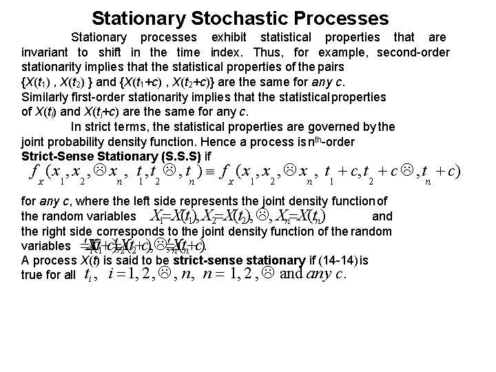
Stationary Stochastic Processes Stationary processes exhibit statistical properties that are invariant to shift in the time index. Thus, for example, second-order stationarity implies that the statistical properties of the pairs {X(t 1) , X(t 2) } and {X(t 1+c) , X(t 2+c)} are the same for any c. Similarly first-order stationarity implies that the statistical properties of X(ti) and X(ti+c) are the same for any c. In strict terms, the statistical properties are governed by the joint probability density function. Hence a process is nth-order Strict-Sense Stationary (S. S. S) if f (x , t , t ) f (x , t c , t c) X 1 2 n 1 2 for any c, where the left side represents the joint density function of the random variables X 1 X(t 1), X 2 X(t 2), , Xn X(tn) and the right side corresponds to the joint density function of the random X X X variables X 1(t 1 c), 2 (t 2 c), , n (tn c). A process X(t) is said to be strict-sense stationary if (14 -14) is true for all ti , i 1, 2 , , n, n 1, 2 , and any c. n

For a first-order strict sense stationary process, from (14 -14) we have f X (x, t) f X (x, t c) (14 -15) for any c. In particular c = – t gives f (x, t) f (x) X X (14 -16) i. e. , the first-order density of X(t) is independent of t. In that case Similarly, for a second-order strict-sense stationary process we have from (14 -14) E[ X (t)] x f ( x)dx , a constant. (14 -17) for any c. For c = – t 2 we get f (x , t , t ) f (x , t c, t 2 c) X 1 2 1 f (x , t , t ) f (x , t t ) X 1 2 1 2 (14 -18)

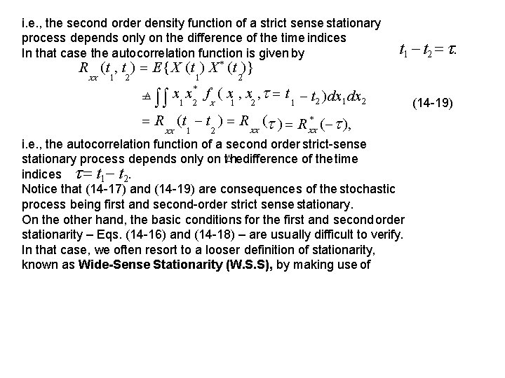
i. e. , the second order density function of a strict sense stationary process depends only on the difference of the time indices In that case the autocorrelation function is given by R (t , t ) E{X (t ) X * (t )} XX 1 2 1 * t 1 t 2 x 1 x 2 f X ( x 1 , x 2 , t 1 t 2 )dx 1 dx 2 * R (t t ) R XX ( ), XX 1 2 i. e. , the autocorrelation function of a second order strict-sense stationary process depends only on t hedifference of the time indices t 1 t 2. Notice that (14 -17) and (14 -19) are consequences of the stochastic process being first and second-order strict sense stationary. On the other hand, the basic conditions for the first and second order stationarity – Eqs. (14 -16) and (14 -18) – are usually difficult to verify. In that case, we often resort to a looser definition of stationarity, known as Wide-Sense Stationarity (W. S. S), by making use of (14 -19)

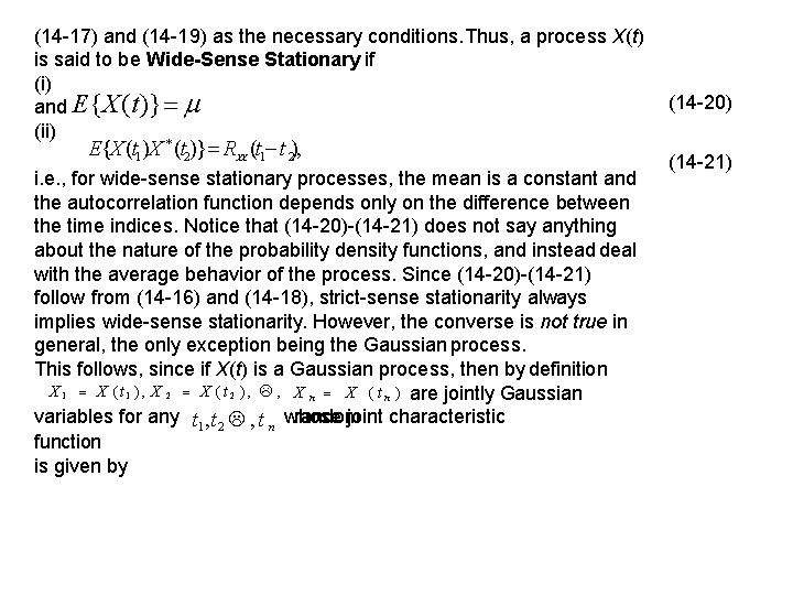
(14 -17) and (14 -19) as the necessary conditions. Thus, a process X(t) is said to be Wide-Sense Stationary if (i) and E{X (t)} (ii) * E{X (t 1)X (t 2)} R (t 1 t 2), XX i. e. , for wide-sense stationary processes, the mean is a constant and the autocorrelation function depends only on the difference between the time indices. Notice that (14 -20)-(14 -21) does not say anything about the nature of the probability density functions, and instead deal with the average behavior of the process. Since (14 -20)-(14 -21) follow from (14 -16) and (14 -18), strict-sense stationarity always implies wide-sense stationarity. However, the converse is not true in general, the only exception being the Gaussian process. This follows, since if X(t) is a Gaussian process, then by definition X 1 X ( t 1 ) , X 2 X ( t 2 ) , , X n X ( t n ) are jointly Gaussian random variables for any t 1, t 2 , t n whose joint characteristic function is given by (14 -20) (14 -21)

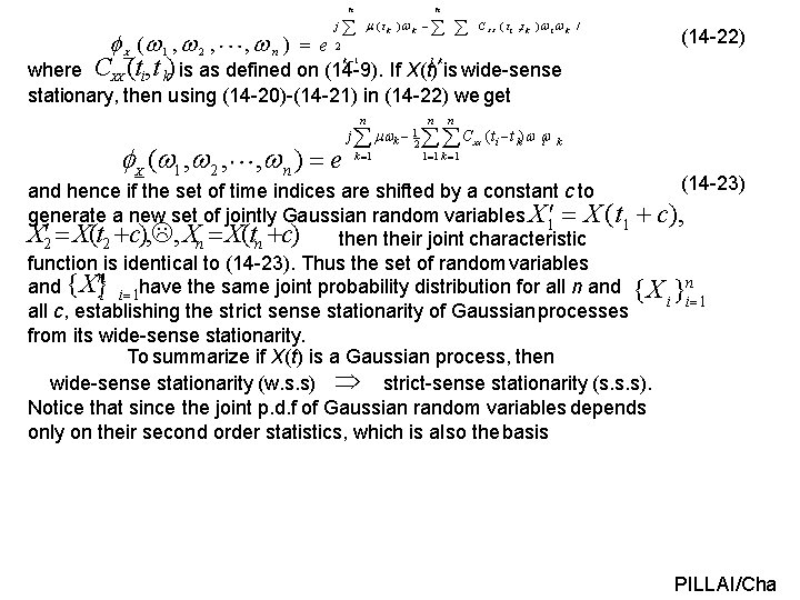
n ( 1 , 2 , j n ( tk ) k C ( ti , t k ) i k / , n ) e 2 where CXX (ti, t k) is as defined on (14 -9). If X(t) is wide-sense stationary, then using (14 -20)-(14 -21) in (14 -22) we get X k 1 ( 1 , 2 , , n ) e (14 -22) l , k n j XX k 1 k 12 n n C XX (ti t k) i k 1 1 k 1 X (14 -23) and hence if the set of time indices are shifted by a constant c to generate a new set of jointly Gaussian random variables X 1 X (t 1 c), X 2 X(t 2 c), , Xn X(tn c) then their joint characteristic function is identical to (14 -23). Thus the set of random variables n and {X}i i 1 have the same joint probability distribution for all n and {X }n i i 1 all c, establishing the strict sense stationarity of Gaussian processes from its wide-sense stationarity. To summarize if X(t) is a Gaussian process, then wide-sense stationarity (w. s. s) strict-sense stationarity (s. s. s). Notice that since the joint p. d. f of Gaussian random variables depends only on their second order statistics, which is also the basis PILLAI/Cha

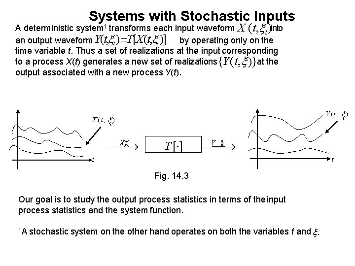
Systems with Stochastic Inputs A deterministic system 1 transforms each input waveform X (t, i )into an output waveform Y(t, i ) T[X (t, i )] by operating only on the time variable t. Thus a set of realizations at the input corresponding to a process X(t) generates a new set of realizations{Y (t, )}at the output associated with a new process Y(t). Y (t , i ) X (t, i ) )t( X T [ ] Y (t) t t Fig. 14. 3 Our goal is to study the output process statistics in terms of the input process statistics and the system function. 1 A stochastic system on the other hand operates on both the variables t and .

Linear Systems: L[ ]represents a linear system if Let L{a 1 X (t 1 ) a 2 X (t 2 )} a 1 L{X (t 1 )} a 2 L{X (t 2 )}. Y (t) L{X (t)} represent the output of a linear system. • Time-Invariant System: L[ ] represents a time-invariant system if (14 -28) (14 -29) • Y (t) L{X (t)} L{X (t t 0 )} Y (t t 0 ) • i. e. , shift in the input results in the same shift (14 -30) in the output also. If L[ ]satisfies both (14 -28) and (14 -30), then it corresponds to a linear time-invariant (LTI) system. • LTI systems can be uniquely represented in terms of their output to a delta function h(t ) (t) LTI h(t) Impulse response of the system t Impulse Fig. 14. 5 Impulse response

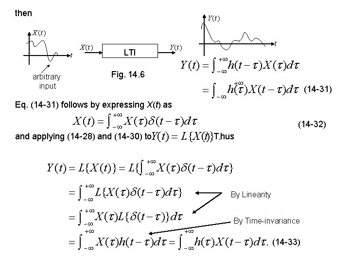
then Y (t ) X (t ) LTI t Y (t) h(t ) X ( )d Fig. 14. 6 arbitrary input t Y (t ) h( ) X (t )d Eq. (14 -31) follows by expressing X(t) as (14 -31) X (t) X ( ) (t )d and applying (14 -28) and (14 -30) to. Y(t) L{X (t)}T. hus (14 -32) Y (t) L{X (t)} L{ X ( ) (t )d } L{X ( ) (t )d } By Linearity X ( )L{ (t )}d By Time-invariance X ( )h(t )d h( ) X (t )d . (14 -33)

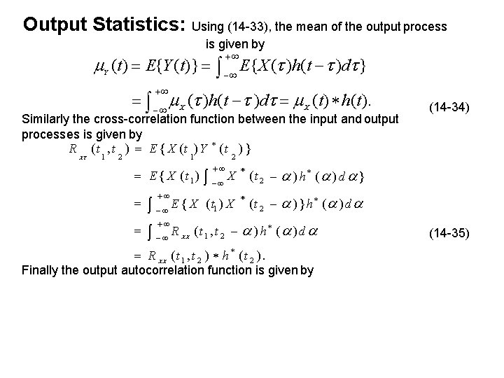
Output Statistics: Using (14 -33), the mean of the output process is given by (t) E{Y (t)} E{X ( )h(t )d } Y X ( )h(t )d X (t) h(t). Similarly the cross-correlation function between the input and output processes is given by R (t , t ) E { X (t )Y * (t )} XY 1 2 1 E { X ( t 1) E { X R XX 2 X * (t 2 ) h * ( ) d } ( t 1 ) X * (t 2 ) } h * ( ) d (t 1 , t 2 ) h * ( ) d R ( t 1 , t 2 ) h * ( t 2 ). Finally the output autocorrelation function is given by XX (14 -34) (14 -35)

R (t , t ) E{Y (t )Y * (t )} YY 1 2 E{ X (t 1 )h( )d Y * (t 2 )} E{X (t )Y * (t )}h( )d 1 2 R XY (t 1 , t 2 )h( )d (14 -36) R XY (t 1 , t 2 ) h(t 1 ), or * RYY (t 1 , t 2 ) R XX (t 1 , t 2 ) h (t 2 ) h(t 1 ). (t) h(t) X (14 -37) Y (a) RXX (t 1 , t 2 ) h*(t 2) XY, tt 12( ) R (b) Fig. 14. 7 h(t 1) RYY (t 1 , t 2 )

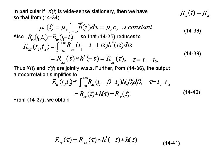
(t) In particular if X(t) is wide-sense stationary, then we have so that from (14 -34) (t) Y X h( )d X X c, a constant. (14 -38) RXX (t 1, t 2 ) RXX (t 1 t 2) so that (14 -35) reduces to * R (t t )h ( )d R XY (t 1 , t 2 ) XX 1 2 Also (14 -39) R XX ( ) h ( ) R XY ( ), t 1 t 2. * Thus X(t) and Y(t) are jointly w. s. s. Further, from (14 -36), the output autocorrelation simplifies to RYY (t 1, t 2) From (14 -37), we obtain R XY (t 1 t 2 )h( )d , t 1 t 2 RXY ( ) h( ) RYY ( ) R XX ( ) h* ( ) h( ). (14 -40) (14 -41) X

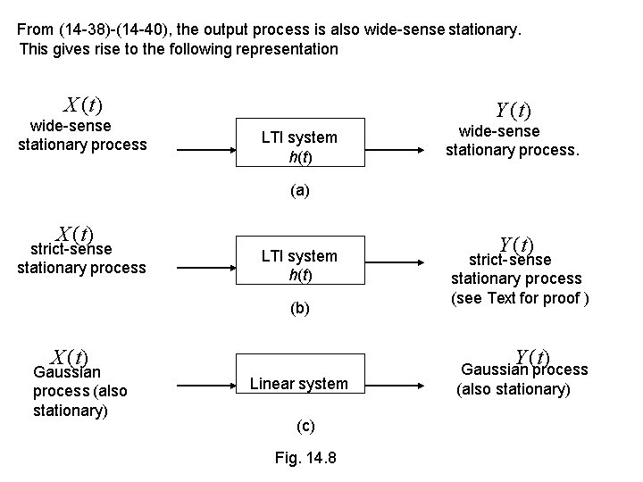
From (14 -38)-(14 -40), the output process is also wide-sense stationary. This gives rise to the following representation X (t) wide-sense stationary process Y (t) LTI system h(t) wide-sense stationary process. (a) X (t) strict-sense stationary process LTI system h(t) (b) X (t) Gaussian process (also stationary) Y (t) strict-sense stationary process (see Text for proof ) Y (t) Linear system (c) Fig. 14. 8 Gaussian process (also stationary)

Discrete Time Stochastic Processes: A discrete time stochastic process Xn = X(n. T) is a sequence of random variables. The mean, autocorrelation and auto-covariance functions of a discrete-time process are gives by n E{X (n. T )} and (14 -57) R(n , n ) E{X (n T ) X * (n T )} 1 2 (14 -58) respectively. As before strict sense stationarity and wide-sense stationarity definitions apply here also. For example, X(n. T) is wide sense stationary if C(n 1 , n 2 ) R(n 1 , n 2 ) n 1 n*2 (14 -59) E{X (n. T )} , a constant (14 -60) and * E[ X {(k n)T}X *{(k)T}] R(n) rn r n (14 -61)

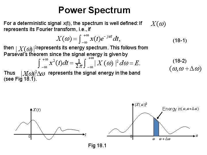
Power Spectrum For a deterministic signal x(t), the spectrum is well defined: If represents its Fourier transform, i. e. , if X ( ) x(t)e j t dt, (18 -1) then | X ( ) |2 represents its energy spectrum. This follows from Parseval’s theorem since the signal energy is given by x (t)dt 2 1 2 2 | X ( ) | d E. Thus | X( )|2 represents the signal energy in the band (see Fig 18. 1). | X ( )|2 X (t ) 0 t 0 Fig 18. 1 (18 -2) ( , ) Energy in( , )

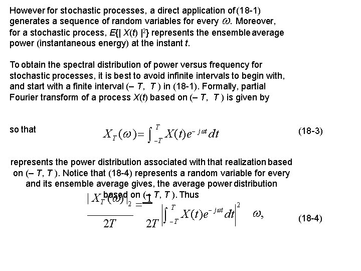
However for stochastic processes, a direct application of (18 -1) generates a sequence of random variables for every . Moreover, for a stochastic process, E{| X(t) |2} represents the ensemble average power (instantaneous energy) at the instant t. To obtain the spectral distribution of power versus frequency for stochastic processes, it is best to avoid infinite intervals to begin with, and start with a finite interval (– T, T ) in (18 -1). Formally, partial Fourier transform of a process X(t) based on (– T, T ) is given by T X T ( ) T X (t)e j t dt so that (18 -3) represents the power distribution associated with that realization based on (– T, T ). Notice that (18 -4) represents a random variable for every and its ensemble average gives, the average power distribution | X based ( ) | on (– 1 T, T ). Thus T 2 T 2 T 2 T T X (t)e j t dt 2 , (18 -4)

T T T ( ) |2 | X 1 E { X (t 1) X P ( ) E T T 2 T 2 T 1 T T j ( t t ) R ( t , t ) e d t 1 d t 2 1 2 T T 2 T T 1 * ( t 2 ) }e j ( t 1 t 2) d t 1 d t 2 2 XX represents the power distribution of X(t) based on (– T, T ). For wide sense stationary (w. s. s) processes, it is possible to further simplify (18 -5). Thus if X(t) is assumed to be w. s. s, then and (18 -5) simplifies to (18 -5) RXX (t 1 , t 2 ) RXX (t 1 t 2 ) Let t 1 t 2 and proceeding as in (14 -24), we get 1 T T j (t 1 t 2) t )e PT ( ) dt 1 dt 2. R (t 2 XX 1 T T 2 T to be the power distribution of the w. s. s. process X(t) based on (– T, T ). Finally letting T in (18 -6), we obtain 1 PT ( ) 2 T 2 T 2 T j R ( )e (2 T | |)d 2 T XX | | )d 0 2 T RXX ( )e j (1 2 T (18 -6)

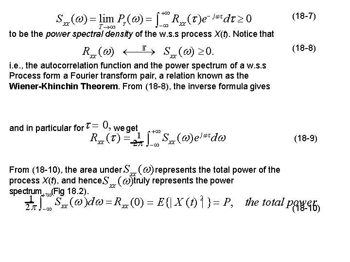
S XX ( ) lim PT ( ) T RXX ( )e j d 0 (18 -7) to be the power spectral density of the w. s. s process X(t). Notice that RXX ( ) FT S XX ( ) 0. (18 -8) i. e. , the autocorrelation function and the power spectrum of a w. s. s Process form a Fourier transform pair, a relation known as the Wiener-Khinchin Theorem. From (18 -8), the inverse formula gives and in particular for 0, we get RXX ( ) 21 S XX ( )e j d From (18 -10), the area under S XX ( ) represents the total power of the process X(t), and hence S ( )truly represents the power XX spectrum. (Fig 18. 2). 1 2 (18 -9) S XX ( )d RXX (0) E{| X (t) 2| } P, the total power. (18 -10)

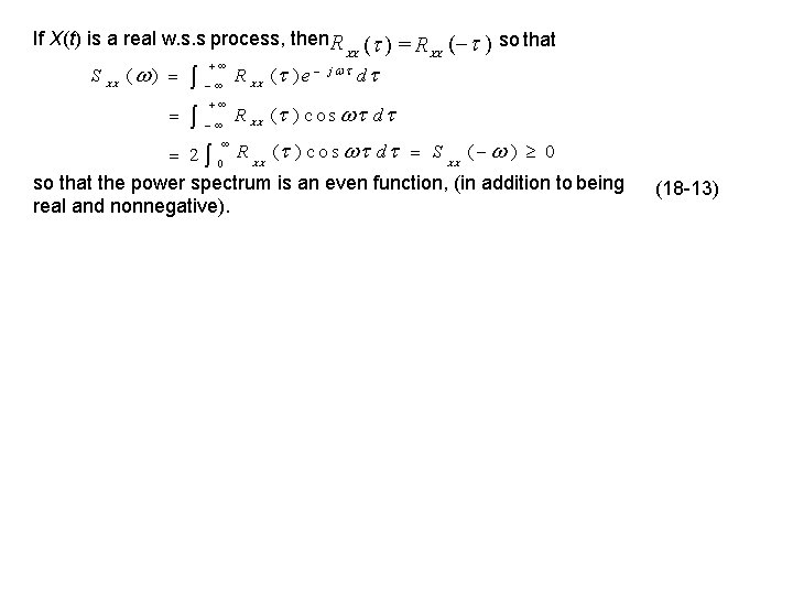
If X(t) is a real w. s. s process, then R ( ) = R ( ) so that XX XX S XX ( ) 2 0 R XX ( ) e j d R XX ( ) c o s d S XX ( ) 0 so that the power spectrum is an even function, (in addition to being real and nonnegative). (18 -13)