NonIntrusive Stochastic Uncertainty Quantification Methods Don Zhang University

Non-Intrusive Stochastic Uncertainty Quantification Methods Don Zhang University of Southern California donzhang@usc. edu Uncertainty Quantification Workshop Tucson, AZ, April 25 -26, 2008

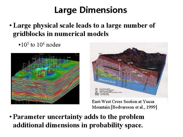
Large Dimensions • Large physical scale leads to a large number of gridblocks in numerical models • 105 to 106 nodes (ft) at Yucca East-West Cross. Distance Section Mountain [Bodvarsson et al. , 1999] • Parameter uncertainty adds to the problem additional dimensions in probability space.

Stochastic Approaches • Two common approaches for quantifying uncertainties associated with subsurface flow simulations: Monte Carlo simulation (MCS) Statistical Moment Equation (SME): Moment equations; Green’s function; Adjoint state • These two types of approaches are complementary.

Intrusive vs. Non-Intrusive Approaches • Moment equation methods are intrusive ØNew governing equations ØExisting deterministic simulators cannot be employed directly • Monte Carlo is non-intrusive: ØDirect sampling ØSame governing equations ØNot efficient • More efficient non-intrusive stochastic approaches are desirable

Stochastic Formulation • SPDE: which has a finite (random) dimensionality. • Weak form solution: where

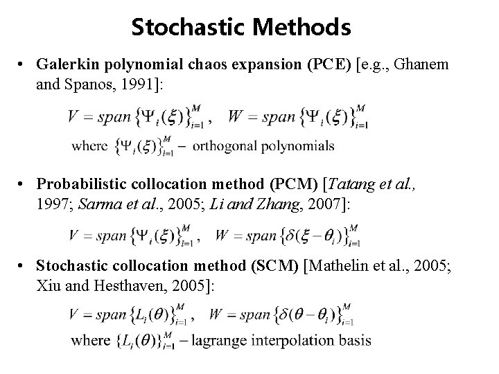
Stochastic Methods • Galerkin polynomial chaos expansion (PCE) [e. g. , Ghanem and Spanos, 1991]: • Probabilistic collocation method (PCM) [Tatang et al. , 1997; Sarma et al. , 2005; Li and Zhang, 2007]: • Stochastic collocation method (SCM) [Mathelin et al. , 2005; Xiu and Hesthaven, 2005]:

Key Components for Stochastic Methods • Random dimensionality of underlying stochastic fields – How to effectively approximate the input random fields with finite dimensions – Karhunen-Loeve and other expansions may be used • Trial function space – How to approximate the dependent random fields – Perturbation series, polynomial chaos expansion, or Lagrange interpolation basis • Test (weighting) function space – How to evaluate the integration in random space? – Intrusive or non-intrusive schemes?

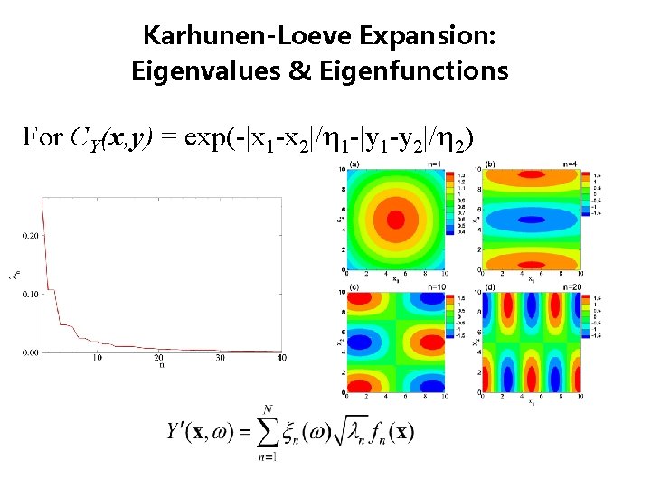
Karhunen-Loeve Expansion: Eigenvalues & Eigenfunctions For CY(x, y) = exp(-|x 1 -x 2|/ 1 -|y 1 -y 2|/ 2)

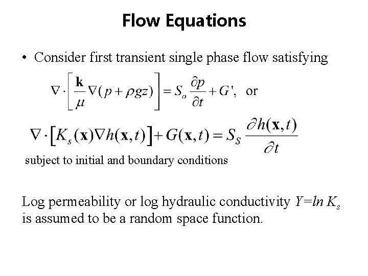
Flow Equations • Consider first transient single phase flow satisfying subject to initial and boundary conditions Log permeability or log hydraulic conductivity Y=ln Ks is assumed to be a random space function.

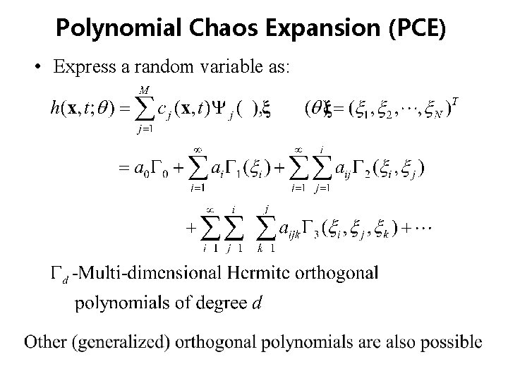
Polynomial Chaos Expansion (PCE) • Express a random variable as:

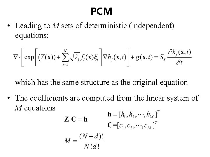
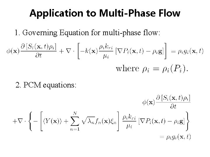
PCM • Leading to M sets of deterministic (independent) equations: which has the same structure as the original equation • The coefficients are computed from the linear system of M equations

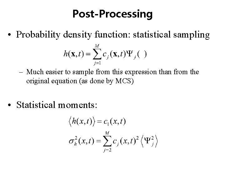
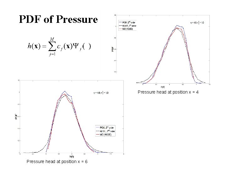
Post-Processing • Probability density function: statistical sampling – Much easier to sample from this expression than from the original equation (as done by MCS) • Statistical moments:

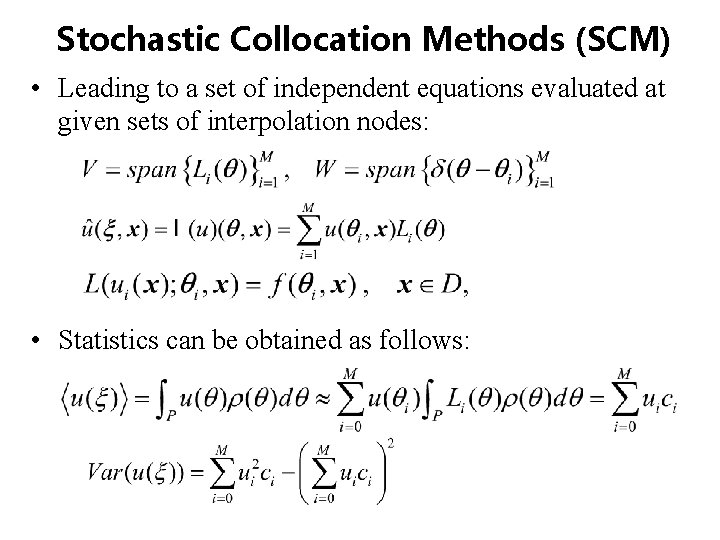
Stochastic Collocation Methods (SCM) • Leading to a set of independent equations evaluated at given sets of interpolation nodes: • Statistics can be obtained as follows:

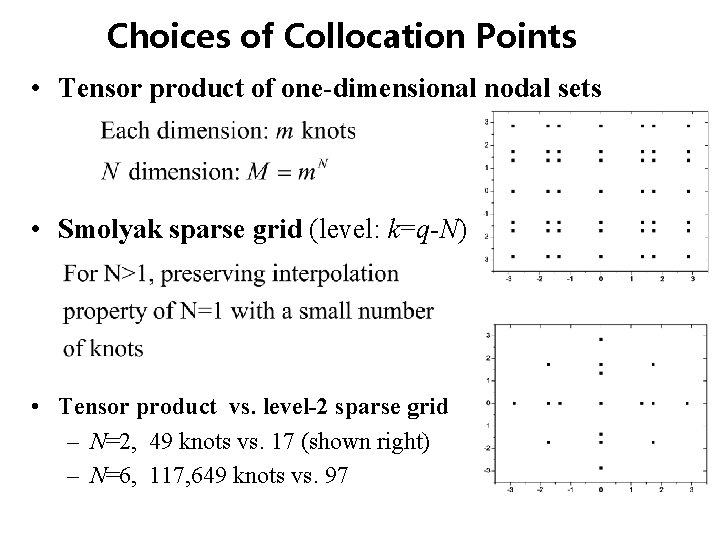
Choices of Collocation Points • Tensor product of one-dimensional nodal sets • Smolyak sparse grid (level: k=q-N) • Tensor product vs. level-2 sparse grid – N=2, 49 knots vs. 17 (shown right) – N=6, 117, 649 knots vs. 97

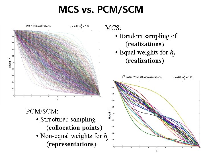
MCS vs. PCM/SCM MCS: • Random sampling of (realizations) • Equal weights for hj (realizations) PCM/SCM: • Structured sampling (collocation points) • Non-equal weights for hj (representations)

PDF of Pressure head at position x = 4 Pressure head at position x = 6

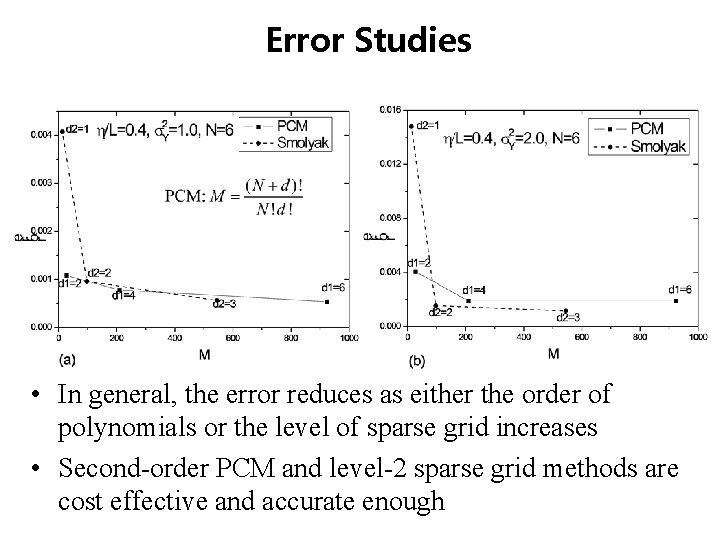
Error Studies • In general, the error reduces as either the order of polynomials or the level of sparse grid increases • Second-order PCM and level-2 sparse grid methods are cost effective and accurate enough

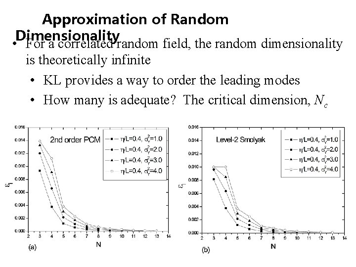
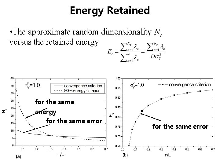
Approximation of Random Dimensionality • For a correlated random field, the random dimensionality is theoretically infinite • KL provides a way to order the leading modes • How many is adequate? The critical dimension, Nc

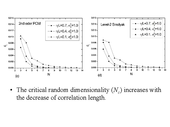
• The critical random dimensionality (Nc) increases with the decrease of correlation length.

Energy Retained • The approximate random dimensionality Nc versus the retained energy for the same error

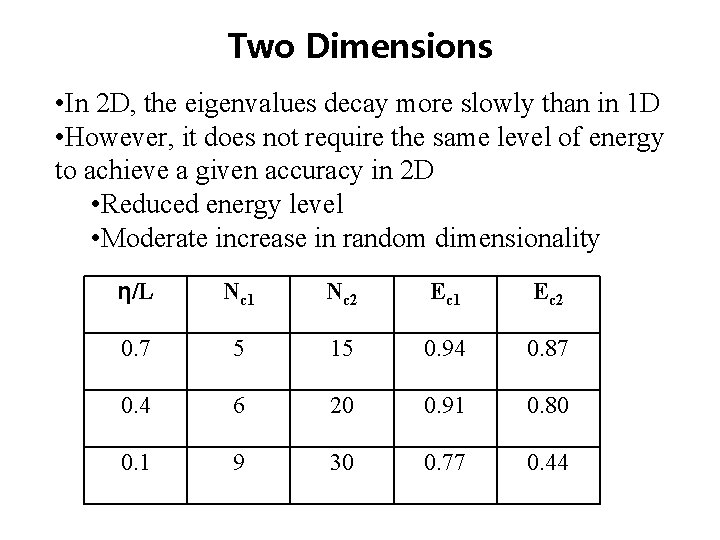
Two Dimensions • In 2 D, the eigenvalues decay more slowly than in 1 D • However, it does not require the same level of energy to achieve a given accuracy in 2 D • Reduced energy level • Moderate increase in random dimensionality η/L Nc 1 Nc 2 Ec 1 Ec 2 0. 7 5 15 0. 94 0. 87 0. 4 6 20 0. 91 0. 80 0. 1 9 30 0. 77 0. 44

Application to Multi-Phase Flow 1. Governing Equation for multi-phase flow: 2. PCM equations:

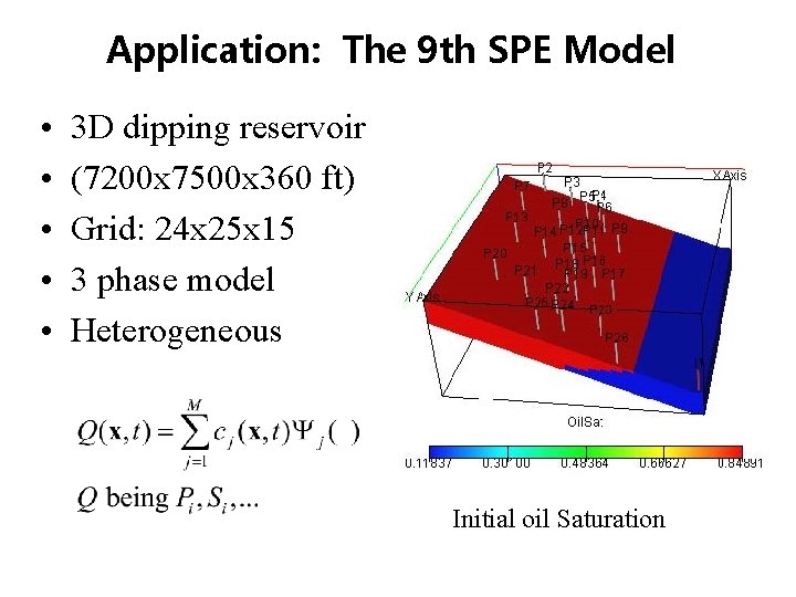
Application: The 9 th SPE Model • • • 3 D dipping reservoir (7200 x 7500 x 360 ft) Grid: 24 x 25 x 15 3 phase model Heterogeneous Initial oil Saturation

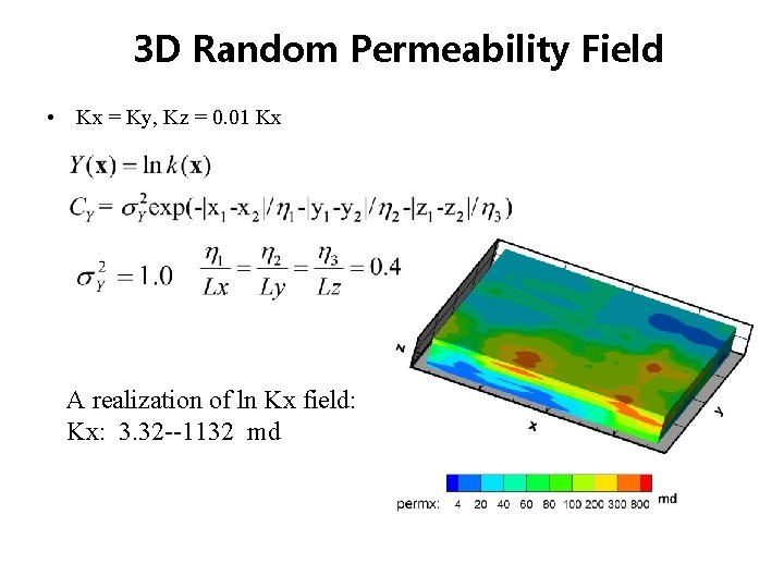
3 D Random Permeability Field • Kx = Ky, Kz = 0. 01 Kx A realization of ln Kx field: Kx: 3. 32 --1132 md

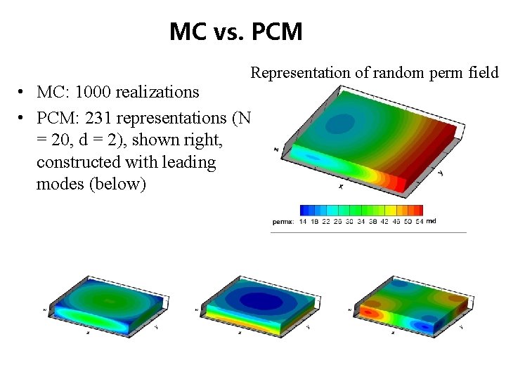
MC vs. PCM Representation of random perm field • MC: 1000 realizations • PCM: 231 representations (N = 20, d = 2), shown right, constructed with leading modes (below)

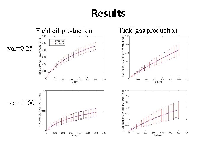
Results Field oil production var=0. 25 var=1. 00 Field gas production

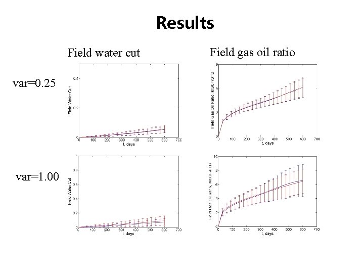
Results Field water cut var=0. 25 var=1. 00 Field gas oil ratio

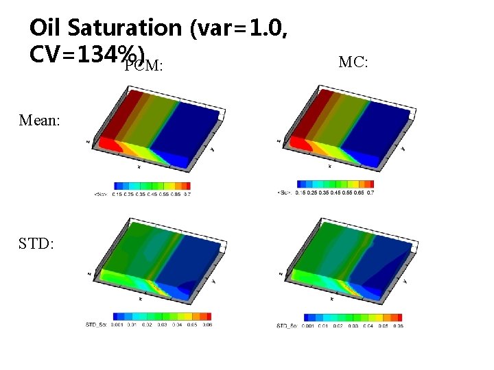
Oil Saturation (var=1. 0, CV=134%) PCM: Mean: STD: MC:

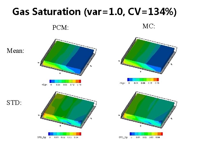
Gas Saturation (var=1. 0, CV=134%) PCM: Mean: STD: MC:

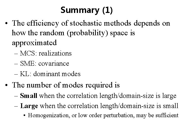
Summary (1) • The efficiency of stochastic methods depends on how the random (probability) space is approximated – MCS: realizations – SME: covariance – KL: dominant modes • The number of modes required is – Small when the correlation length/domain-size is large – Large when the correlation length/domain-size is small • Homogenization, or low order perturbation, may be sufficient

Summary (2) • The relative effectiveness of PCE and PCM/SCM depends on how their expansion coefficients are evaluated – PCE: Coupled equations – PCM & SCM: Independent equations with the same structure as the original one • PCM & SCM: Promising for large scale problems

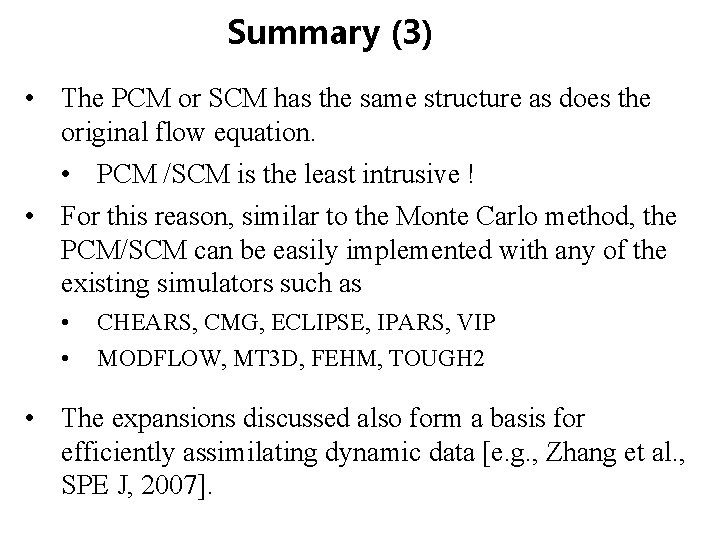
Summary (3) • The PCM or SCM has the same structure as does the original flow equation. • PCM /SCM is the least intrusive ! • For this reason, similar to the Monte Carlo method, the PCM/SCM can be easily implemented with any of the existing simulators such as • • CHEARS, CMG, ECLIPSE, IPARS, VIP MODFLOW, MT 3 D, FEHM, TOUGH 2 • The expansions discussed also form a basis for efficiently assimilating dynamic data [e. g. , Zhang et al. , SPE J, 2007].

Acknowledgment Financial Supports: NSF; ACS; DOE; Industrial Consortium “OU-CEM”

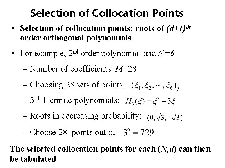
Selection of Collocation Points • Selection of collocation points: roots of (d+1)th order orthogonal polynomials • For example, 2 nd order polynomial and N=6 – Number of coefficients: M=28 – Choosing 28 sets of points: – 3 rd Hermite polynomials: – Roots in decreasing probability: – Choose 28 points out of The selected collocation points for each (N, d) can then be tabulated.