Stochastic Process for MS CSE 5403 Stochastic Process

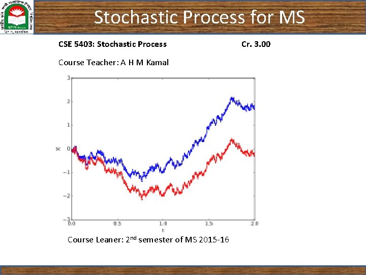
Stochastic Process for MS CSE 5403: Stochastic Process Course Teacher: A H M Kamal Course Leaner: 2 nd semester of MS 2015 -16 Cr. 3. 00

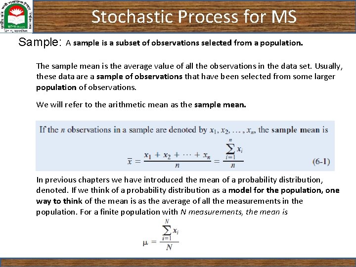
Stochastic Process for MS Sample: A sample is a subset of observations selected from a population. The sample mean is the average value of all the observations in the data set. Usually, these data are a sample of observations that have been selected from some larger population of observations. We will refer to the arithmetic mean as the sample mean. In previous chapters we have introduced the mean of a probability distribution, denoted. If we think of a probability distribution as a model for the population, one way to think of the mean is as the average of all the measurements in the population. For a finite population with N measurements, the mean is

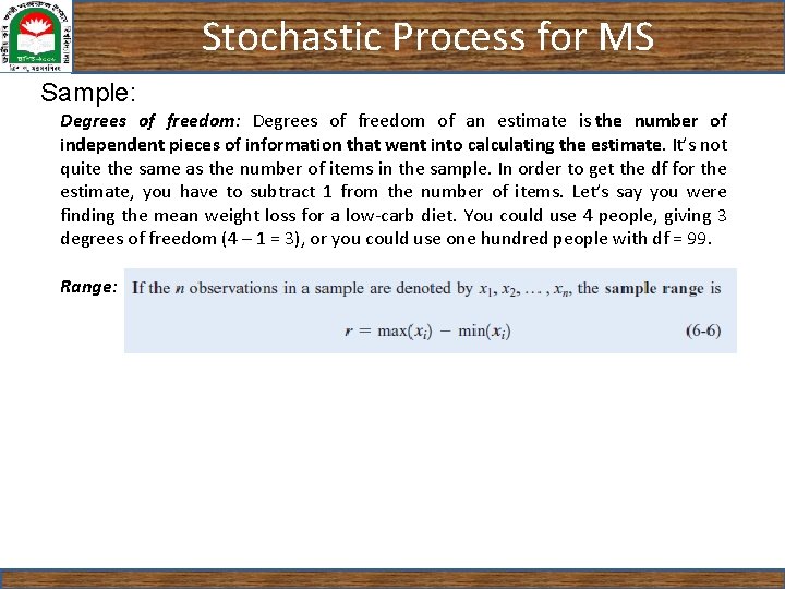
Stochastic Process for MS Sample: Degrees of freedom: Degrees of freedom of an estimate is the number of independent pieces of information that went into calculating the estimate. It’s not quite the same as the number of items in the sample. In order to get the df for the estimate, you have to subtract 1 from the number of items. Let’s say you were finding the mean weight loss for a low-carb diet. You could use 4 people, giving 3 degrees of freedom (4 – 1 = 3), or you could use one hundred people with df = 99. Range:

Stochastic Process for MS Sample: For statistical methods to be valid, the sample must be representative of the population. It is often * tempting to select the observations that are most convenient as the sample. * bias into the sample To avoid these difficulties, it is desirable to select a random sample as the result of some chance mechanism. Consequence: # the selection of a sample is a random experiment # each observation in the sample is the observed value of a random variable # The observations in the population determine the probability distribution of the random variable.

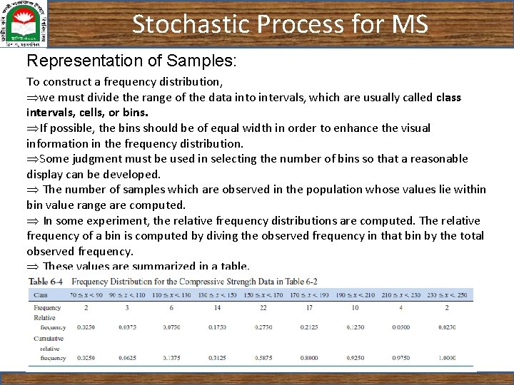
Stochastic Process for MS Representation of Samples: To construct a frequency distribution, Þwe must divide the range of the data into intervals, which are usually called class intervals, cells, or bins. ÞIf possible, the bins should be of equal width in order to enhance the visual information in the frequency distribution. ÞSome judgment must be used in selecting the number of bins so that a reasonable display can be developed. Þ The number of samples which are observed in the population whose values lie within bin value range are computed. Þ In some experiment, the relative frequency distributions are computed. The relative frequency of a bin is computed by diving the observed frequency in that bin by the total observed frequency. Þ These values are summarized in a table.

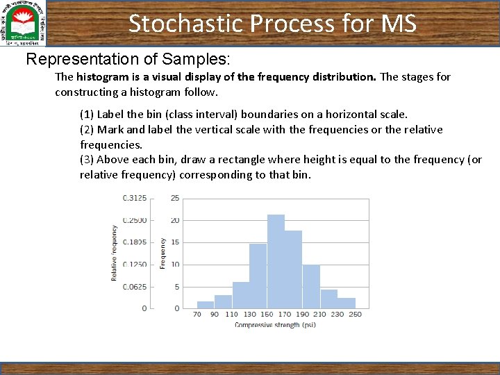
Stochastic Process for MS Representation of Samples: The histogram is a visual display of the frequency distribution. The stages for constructing a histogram follow. (1) Label the bin (class interval) boundaries on a horizontal scale. (2) Mark and label the vertical scale with the frequencies or the relative frequencies. (3) Above each bin, draw a rectangle where height is equal to the frequency (or relative frequency) corresponding to that bin.

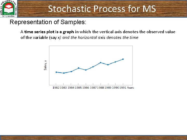
Stochastic Process for MS Representation of Samples: A time series plot is a graph in which the vertical axis denotes the observed value of the variable (say x) and the horizontal axis denotes the time

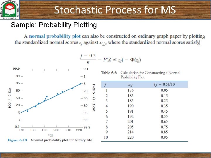
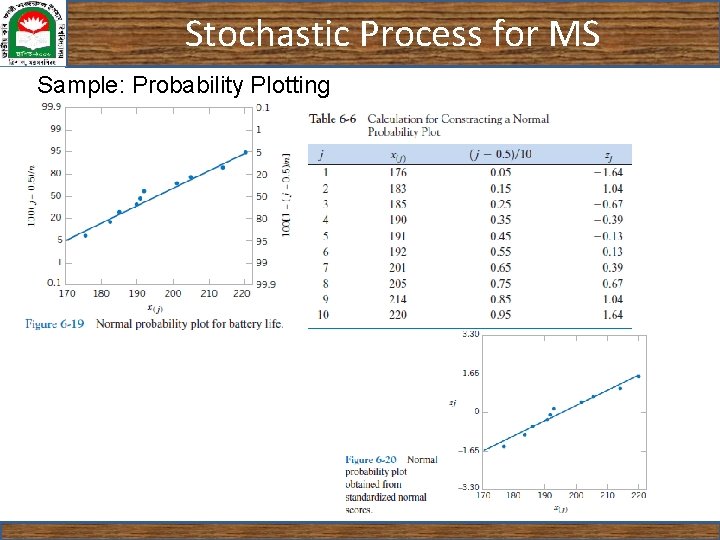
Stochastic Process for MS Sample: Probability Plotting Some of the visual displays we have used earlier, such as the histogram, can provide insight about the form of the underlying distribution. However, histograms are usually not really reliable indicators of the distribution form unless the sample size is very large. Probability plotting is a graphical method for determining whether sample data conform to a hypothesized distribution based on a subjective visual examination of the data. To construct a probability plot, the observations in the sample are first ranked from smallest to largest. That is, the sample x 1, x 2, … …, xn is arranged as where x(1), x(2), … …, x(n) is the smallest observation, x(2) is the second smallest observation, and so forth, with x(n) the largest. The ordered observations x( j) are then plotted against their observed cumulative frequency ( j -0. 5)/n on the appropriate probability paper. If the hypothesized distribution adequately describes the data, the plotted points will fall approximately along a straight line; if the plotted points deviate significantly from a straight line, the hypothesized model is not appropriate.

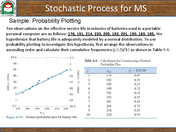
Stochastic Process for MS Sample: Probability Plotting Ten observations on the effective service life in minutes of batteries used in a portable personal computer are as follows: 176, 191, 214, 220, 205, 192, 201, 190, 183, 185. We hypothesize that battery life is adequately modeled by a normal distribution. To use probability plotting to investigate this hypothesis, first arrange the observations in ascending order and calculate their cumulative frequencies (j-0. 5)/10 as shown in Table 6 -6. The pairs of values x(j) and (j-0. 5)/10 are now plotted on normal probability paper. This plot is shown in Fig. 6 -19. Most normal probability paper plots 100(j-0. 5)/n on the left vertical scale and 100[1 - (j-0. 5)/n] on the right vertical scale, with the variable value plotted on the horizontal scale. A straight line, chosen subjectively, has been drawn through the plotted points. In drawing the straight line, you should be influenced more by the points near the middle of the plot than by the extreme points. A good rule of thumb is to draw the line approximately between the 25 th and 75 th percentile points. This is how the line in Fig. 6 -19 was determined.

Stochastic Process for MS Sample: Probability Plotting Ten observations on the effective service life in minutes of batteries used in a portable personal computer are as follows: 176, 191, 214, 220, 205, 192, 201, 190, 183, 185. We hypothesize that battery life is adequately modeled by a normal distribution. To use probability plotting to investigate this hypothesis, first arrange the observations in ascending order and calculate their cumulative frequencies (j-0. 5)/10 as shown in Table 6 -6.

Stochastic Process for MS Sample: Probability Plotting

Stochastic Process for MS Sample: Probability Plotting

Stochastic Process for MS Sample: Probability Plotting