Chapter 12 Inventory Models Introduction Inventory management is

- Slides: 52

Chapter 12 Inventory Models

Introduction • Inventory management is one of the most important decisions faced by many companies. • They all face two competing pressures. – The first is the pressure to have enough inventory on hand. • The most obvious reason for this is that they do not want to run out of products that customers demand. • Another prominent reason, however, is the fixed cost of ordering or producing, as discussed throughout this chapter. • If a fixed cost is incurred each time the company orders from its supplier, or a fixed cost is incurred each time a manufacturer produces a batch, where this cost does not depend on the order or batch size, the company has an incentive to place large orders or produce large batches to minimize its annual fixed costs Winston/Albright Practical Management Science, 4 e South-Western/Cengage Learning © 2012 Thomson/South-Western 2007 ©

Introduction continued – The second pressure related to inventory management is the pressure to carry as little inventory as possible. • The most obvious reasons for this are the cost of storing items and the interest costs involved in tying up money in inventory. • These two competing pressures are at the heart of most inventory models. • The balance is typically not easy to find, so they need models to determine the best ordering (or production) policy. Winston/Albright Practical Management Science, 4 e South-Western/Cengage Learning © 2012 Thomson/South-Western 2007 ©

Introduction continued • An inventory problem can usually be broken up into two parts: 1. how much to order on each ordering opportunity and 2. when to order. • When customer demand is assumed to be known, the resulting models are called deterministic models. • A more realistic situation occurs when customer demand is uncertain. In this case, the decision on when to place orders becomes more difficult. These more difficult problems require probabilistic inventory models. Winston/Albright Practical Management Science, 4 e South-Western/Cengage Learning © 2012 Thomson/South-Western 2007 ©

Categories of inventory models • Researchers have analyzed many inventory models, both deterministic and probabilistic. • We discuss only the most basic of these models, which have been used extensively in real applications. • We begin by discussing several important issues and introducing some terminology. • Keep in mind, however, that the possible number of real-world situations that require inventory management is virtually unlimited. • We list only some of the factors that are common to these situations. Winston/Albright Practical Management Science, 4 e South-Western/Cengage Learning © 2012 Thomson/South-Western 2007 ©

Deterministic vs. probabilistic models • In deterministic models, all inputs to the problem, particularly customer demand, are assumed to be known when the decisions are made. – In reality, a company must always forecast future demands with some type of forecasting model. – The outputs of this forecasting model might include a mean demand a standard deviation of demand. – In deterministic models, however, only the mean is used, and any information about the uncertainty, such as the standard deviation, is ignored. – This makes the resulting models simpler, but usually less realistic. Winston/Albright Practical Management Science, 4 e South-Western/Cengage Learning © 2012 Thomson/South-Western 2007 ©

Deterministic vs. probabilistic models continued • Probabilistic models use this information about uncertainty explicitly. • They are typically more difficult to analyze, but they tend to produce better decisions, especially when the level of uncertainty is high. Winston/Albright Practical Management Science, 4 e South-Western/Cengage Learning © 2012 Thomson/South-Western 2007 ©

External vs. internal demand • A second factor in inventory modeling is whether demand for the product is generated externally or internally. • External demand (or independent demand) occurs when the company that sells the product cannot directly control the extent or the timing of customer demand. • In contrast, internal demand (or dependent demand) occurs in most assembly and manufacturing processes. Winston/Albright Practical Management Science, 4 e South-Western/Cengage Learning © 2012 Thomson/South-Western 2007 ©

Ordering vs. production • A third factor in inventory modeling is whether the company orders the products from a supplier or produces them internally. • If the products are ordered, then there is typically an order lead time, the time elapsed from when the order is placed until it arrives. • In ordering models, there is also usually a fixed cost (also called a setup or ordering cost) each time an order is placed, where this cost is independent of the order quantity. Winston/Albright Practical Management Science, 4 e South-Western/Cengage Learning © 2012 Thomson/South-Western 2007 ©

Ordering vs. production continued • In contrast, if products are produced internally, there is also a lead time, the time it takes to produce a batch of items. This time is determined by a production rate. • As in ordering models, there can also be a setup cost each time a batch is produced, where this cost is independent of the batch size. Winston/Albright Practical Management Science, 4 e South-Western/Cengage Learning © 2012 Thomson/South-Western 2007 ©

Continuous vs. periodic review • A fourth factor in inventory modeling is whether inventory is reviewed continuously or periodically. • In continuous review models, the inventory is monitored continually and orders can be placed at any time. • Typically, there is a reorder point - a specific inventory level—so that when the inventory on hand reaches this reorder point, an order is placed immediately. Winston/Albright Practical Management Science, 4 e South-Western/Cengage Learning © 2012 Thomson/South-Western 2007 ©

Continuous vs. periodic review continued • In contrast, in periodic review models, there is some standard time, such as every Monday morning, when the inventory is reviewed and ordering decisions are made. • Except possibly for emergency orders, these are the only times when orders are placed. • Continuous review models can certainly be implemented, given today’s computerized access to inventory levels in real time, and these models can result in lower annual costs than periodic review models. • However, when a company stocks many products (hundreds or even thousands), it is often more convenient to use periodic review. Winston/Albright Practical Management Science, 4 e South-Western/Cengage Learning © 2012 Thomson/South-Western 2007 ©

Single-product vs. multipleproduct models • A final factor in inventory modeling concerns the number of products involved. • Models that consider only a single product are conceptually and mathematically simpler, so we initially analyze single-product models. • However, most companies have many different products that must be considered simultaneously. • If the company orders these items from a supplier, it may be wise to synchronize the orders in some way to minimize ordering costs. Winston/Albright Practical Management Science, 4 e South-Western/Cengage Learning © 2012 Thomson/South-Western 2007 ©

Types of costs in inventory models • Companies face a number of costs when they manage inventories. Although the types of costs vary depending on the company and the situation, the following costs are typical. • Ordering (setup) cost is the fixed cost incurred every time an order is placed or a batch is produced, independent of the amount ordered or produced. – This ordering cost includes the cost of paperwork and billing each time an order is placed and could include other costs as well, such as paying a truck driver to deliver the order to the company’s warehouse. – If the product is produced rather than ordered, this cost can include the cost to set up equipment. Winston/Albright Practical Management Science, 4 e South-Western/Cengage Learning © 2012 Thomson/South-Western 2007 ©

Types of costs in inventory models continued • The unit purchasing (or production) cost is the cost for each additional unit purchased or produced (often referred to as the variable cost). • The holding (or carrying) cost is the cost that motivates the company to keep less inventory on hand. – This cost generally has two components, the financial holding cost and the nonfinancial holding cost. The nonfinancial holding cost is usually the cost of storing the product. Winston/Albright Practical Management Science, 4 e South-Western/Cengage Learning © 2012 Thomson/South-Western 2007 ©

Types of costs in inventory models continued • It is often important to measure the cost of running out of inventory. This shortage (or penalty) cost is a difficult cost to measure. – At one extreme, there are lost sales models, where any demands that occur when inventory is zero are lost; these customers take their business elsewhere. – At the other extreme, there are complete backlogging models, where demands that occur when inventory is zero are satisfied as soon as a new order arrives. – Both of these models—or any in between, called partial backlogging models—have negative effects for the company. Winston/Albright Practical Management Science, 4 e South-Western/Cengage Learning © 2012 Thomson/South-Western 2007 ©

Types of costs in inventory models continued • Finally, there is the selling price of the product and the resulting revenue to the company. – In many situations, the revenue is a fixed amount that is not affected by any ordering decisions. – This occurs when the selling price remains constant and the company intends to satisfy all demand eventually. Winston/Albright Practical Management Science, 4 e South-Western/Cengage Learning © 2012 Thomson/South-Western 2007 ©

Economic order quantity (EOQ) models • We first examine a class of models called economic order quantity (EOQ) models. These are the most basic of all the inventory planning models. • We begin by studying the most basic EOQ model. Then we examine several interesting variations of this basic model. All of these models make the following assumptions: – A company orders a single product from a supplier and sells this product to its customers. Winston/Albright Practical Management Science, 4 e South-Western/Cengage Learning © 2012 Thomson/South-Western 2007 ©

Economic order quantity (EOQ) models continued – Orders can be placed at any time (continuous review). – There is a constant, known demand rate for the product, usually expressed in units per year (annual demand). – There is a constant, known lead time for delivery of the product from the supplier. – There is a fixed ordering cost each time the product is ordered, independent of the size of the order. – The price the company charges for the product is fixed. – The annual holding cost is proportional to the average amount of inventory on hand. Winston/Albright Practical Management Science, 4 e South-Western/Cengage Learning © 2012 Thomson/South-Western 2007 ©

The basic EOQ model • The most basic EOQ model adds the following two assumptions. – No stockouts are allowed; that is, the company never allows itself to run out of inventory. – The unit cost of purchasing the product from the supplier is constant. In particular, no quantity discounts are available. • These assumptions have important implications. – Because the demand rate and lead time are assumed to be known, the company can ensure that it always has enough on hand to meet demand on time. Winston/Albright Practical Management Science, 4 e South-Western/Cengage Learning © 2012 Thomson/South-Western 2007 ©

The basic EOQ model continued • The main decision is whether to order small amounts frequently or to order large amounts infrequently. • The former results in large fixed costs and small holding costs (less inventory on hand), whereas the latter results in the opposite. • The EOQ analysis balances these two competing forces. • The basic EOQ model is demonstrated in Example 12. 1 Winston/Albright Practical Management Science, 4 e South-Western/Cengage Learning © 2012 Thomson/South-Western 2007 ©

EOQ model with quantity discounts • Example 12. 2 illustrates one of many possible variations of the basic EOQ model. • In this variation, the company placing the order can obtain quantity discounts from its supplier. Winston/Albright Practical Management Science, 4 e South-Western/Cengage Learning © 2012 Thomson/South-Western 2007 ©

EOQ model with shortages allowed • A key assumption in the basic EOQ model is that the company decides, as a matter of policy, not to allow any shortages. • Because the demand rate and the lead time are known, the ordering can be done so that an order arrives just as the inventory level reaches zero. • This means that it is possible to prevent shortages from occurring. • However, it might be in the company’s best interests to allow a few shortages if the penalty for a shortage is not too large. Winston/Albright Practical Management Science, 4 e South-Western/Cengage Learning © 2012 Thomson/South-Western 2007 ©

EOQ models with shortages allowed continued • First, are shortages backlogged or are these demands lost? • And what about the penalty cost for a shortage? • Does the penalty relate only to the number of units short per year or also to the amount of time the shortages last? • Whatever type of shortage cost is assumed, the practical difficulty is then assessing a specific dollar value for this cost. Winston/Albright Practical Management Science, 4 e South-Western/Cengage Learning © 2012 Thomson/South-Western 2007 ©

EOQ models with shortages allowed continued • Example 12. 3 illustrates a complete backlog model where the penalty cost is charged per unit short per amount of time short. • In this case, the annual penalty cost is a constant p multiplied by the product of the average number of units backlogged and the average amount of time a customer has to wait for a backlogged unit. • The constant p is the penalty cost charged for each customer who has to wait one unit of time for one backlogged item. Winston/Albright Practical Management Science, 4 e South-Western/Cengage Learning © 2012 Thomson/South-Western 2007 ©

Reducing the setup cost • There has been a lot of talk in recent years about striving for zero inventory. • The argument is that the less inventory a company carries, the more efficiently it is operating its business. • The question is whether this argument can be justified from an economic point of view, at least in the context of the EOQ models we have been discussing. • One possible answer to this question is to reconsider whether the setup cost is really fixed. Winston/Albright Practical Management Science, 4 e South-Western/Cengage Learning © 2012 Thomson/South-Western 2007 ©

Reducing the setup cost continued • There are two modeling problems here. – The first is to choose a reasonable form for the function f(K). – The second is to find a way to turn a one-time investment cost, f (K), into an equivalent annual cost, so that the cost of reducing the setup cost is comparable to the annual operating costs we have been discussing. • Putting all of this together, the total annual cost to the company is f (K)i plus the annual operating cost from any of the previous models. • In addition to any previous decision variables, such as Q, K must be chosen, subject to the constraint K K 0. • Example 12. 4 illustrates the procedure. Winston/Albright Practical Management Science, 4 e South-Western/Cengage Learning © 2012 Thomson/South-Western 2007 ©

Synchronizing orders with several products • Until now, all models have considered a single product. • If the company orders several products, it could calculate the EOQ for each product and order them according to separate schedules. • However, there might be economies, particularly reduced setup costs, from synchronizing the orders so that several products are ordered simultaneously. • This should be particularly attractive for products that come from the same supplier. Winston/Albright Practical Management Science, 4 e South-Western/Cengage Learning © 2012 Thomson/South-Western 2007 ©

Synchronizing orders with several products continued • We develop a model in this section that takes advantage of synchronization, and we compare it to the “individual EOQs” policy that uses no synchronization. • Although this model can be developed for any number of products, we keep things relatively simple by assuming that there are only two products. • This model is shown in Example 12. 5. Winston/Albright Practical Management Science, 4 e South-Western/Cengage Learning © 2012 Thomson/South-Western 2007 ©

More than two products • Virtually the same spreadsheet could be used for more than two products, provided that we make a simplifying assumption. • This assumption is that a setup cost reduction is available only when the company places an order for all of the products simultaneously. • Unfortunately, it is probably more realistic to assume that there is a setup cost reduction when any subset of products is ordered simultaneously. • If we allow this possibility, however, and then try to optimize over all possible synchronizations, the problem becomes difficult to model in a spreadsheet. • Therefore, we do not pursue this multiple-product model any further here. Winston/Albright Practical Management Science, 4 e South-Western/Cengage Learning © 2012 Thomson/South-Western 2007 ©

Probabilistic inventory models • In most situations, companies that make ordering and production decisions face uncertainty about the future. • Probably the most common and important element of uncertainty is customer demand, but there can be others. • The company that faces uncertainty has three basic options: use best guess, develop a nonsimulation model, or develop a simulation model. • The advantage of a simulation model is that it is relatively easy to develop, regardless of the complexity of the problem. The disadvantage is that it can be difficult, or at least time-consuming, to find optimal ordering policies from a simulation. Winston/Albright Practical Management Science, 4 e South-Western/Cengage Learning © 2012 Thomson/South-Western 2007 ©

Newsvendor model • The newsvendor model is one of the simplest probabilistic inventory models, but it is also a very important one. • It occurs whenever a company must place a onetime order for a product and then wait to see the demand for the product. • The assumption is that after this demand occurs, the product is no longer valuable. • Given the single chance to order, the company needs to balance the cost of ordering too much versus the cost of not ordering enough. Winston/Albright Practical Management Science, 4 e South-Western/Cengage Learning © 2012 Thomson/South-Western 2007 ©

Newsvendor model continued • To put this problem in a fairly general setting, let cover and cunder, respectively, be the cost of having one more unit or one fewer unit on hand than demand. • Now let D be the random demand. – We assume that D has a cumulative probability distribution F(x), so that for any potential demand x, F(x) is the probability P(D < x) that D is less than or equal to x. Winston/Albright Practical Management Science, 4 e South-Western/Cengage Learning © 2012 Thomson/South-Western 2007 ©

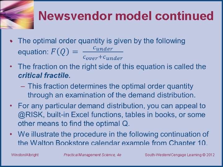
Newsvendor model continued • Winston/Albright Practical Management Science, 4 e South-Western/Cengage Learning © 2012 Thomson/South-Western 2007 ©

Example 12. 6: Background information • Recall that Walton Bookstore buys calendars for $7. 50, sells them at the regular price of $10, and gets a refund of $2. 50 for all calendars that cannot be sold. • As in Example 10. 3 of Chapter 10, Walton estimates that demand for the calendar has a triangular distribution with minimum, most likely, and maximum values equal to 100, 175, and 300, respectively. • How many calendars should Walton order to maximize expected profit? Winston/Albright Practical Management Science, 4 e South-Western/Cengage Learning © 2012 Thomson/South-Western 2007 ©

The (R, Q) ordering policy • The previous subsection analyzed a one-time ordering decision, which is relevant for a product such as a newspaper or a fashion item that quickly goes out of style. • We now examine an ordering decision for a product with sales that continue into the indefinite future. • Consider this: the probability distribution of demand in any month, say, is always the same, but the actual demands in different months can be different because of randomness. Practical Management Science, 4 e Winston/Albright South-Western/Cengage Learning © 2012 Thomson/South-Western 2007 ©

The (R, Q) ordering policy continued • As with the deterministic EOQ model, the company must make two decisions: when to order and how much to order. • We assume that it uses a popular type of policy, called an (R, Q) policy, where R is the reorder point and Q is the order quantity. • Under this policy, the company continually monitors its inventory. When inventory drops to R or below, the company places an order for Q units. Winston/Albright Practical Management Science, 4 e South-Western/Cengage Learning © 2012 Thomson/South-Western 2007 ©

The (R, Q) ordering policy continued • When a company chooses the reorder point R, it must take into account the effects of running out of inventory. • If the company believes shortages are very expensive or undesirable, it should choose a relatively large value of R. • This leads to a relatively large level of safety stock, the expected amount of inventory left over - the cushion - by the time the next order arrives. Winston/Albright Practical Management Science, 4 e South-Western/Cengage Learning © 2012 Thomson/South-Western 2007 ©

The (R, Q) ordering policy continued • On the other hand, if shortages are not considered too expensive or undesirable, the company can afford to use a lower value of R, with a smaller resulting level of safety stock. • As in the newsvendor model, we show to determine an appropriate trade-off between leftovers and shortages. Winston/Albright Practical Management Science, 4 e South-Western/Cengage Learning © 2012 Thomson/South-Western 2007 ©

The (R, Q) ordering policy continued • To specify an (R, Q) policy, we must also determine the appropriate order quantity Q. • It turns out that the choices of R and Q can be made almost independently. – The choice of R depends largely on how shortage costs (or customer service) are measured, whereas the choice of Q depends mostly on the same cost factors considered in the deterministic EOQ models. • Fortunately, it is possible to develop a Solver model that determines Q and R simultaneously, as illustrated in the example 12. 7. Winston/Albright Practical Management Science, 4 e South-Western/Cengage Learning © 2012 Thomson/South-Western 2007 ©

Random lead times • We have assumed that the lead time for orders is a known quantity. • It is not difficult to modify the analysis for the case where the lead time L is random. • This is important, because it is not at all uncommon in real applications for ordering lead times to be uncertain – suppliers might not be able to deliver according to a precise schedule. Winston/Albright Practical Management Science, 4 e South-Western/Cengage Learning © 2012 Thomson/South-Western 2007 ©

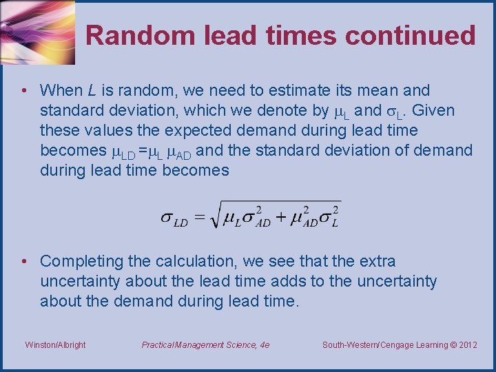
Random lead times continued • When L is random, we need to estimate its mean and standard deviation, which we denote by L and L. Given these values the expected demand during lead time becomes LD = L AD and the standard deviation of demand during lead time becomes • Completing the calculation, we see that the extra uncertainty about the lead time adds to the uncertainty about the demand during lead time. Winston/Albright Practical Management Science, 4 e South-Western/Cengage Learning © 2012 Thomson/South-Western 2007 ©

Random lead times continued • Once we use these formulas to obtain LD and LD, we find the optimal (R, Q) exactly as in the nonrandom lead time case. • When the lead time is uncertain, a company needs to order earlier, which means larger safety stock and higher inventory holding costs. Winston/Albright Practical Management Science, 4 e South-Western/Cengage Learning © 2012 Thomson/South-Western 2007 ©

Ordering simulation models • As problems become more complex, the required mathematical models become too difficult for most managers to comprehend. • In fact, mathematical models do not even exist for many realistic problems. • Therefore, it is useful to turn to simulation, where virtually anything is allowed. • Simulation allows you to combine assumptions about uncertain quantities and ordering policies and then play out the events as they occur through time. • The following example illustrates a somewhat more ambitious ordering simulation. • It describes a type of ordering policy, an (s, S) policy, that is commonly used in periodic review situations. • Example 12. 8 is typical. Winston/Albright Practical Management Science, 4 e South-Western/Cengage Learning © 2012 Thomson/South-Western 2007 ©

Supply chain models • One of today’s hottest areas of interest, both for academics and business managers, is supply chain management. • This refers to the entire process of getting materials from suppliers, transforming them into finished products, and ultimately getting the finished products to customers. • Efficient supply chains have become a requirement in most industries. Without them, companies cannot compete successfully. Winston/Albright Practical Management Science, 4 e South-Western/Cengage Learning © 2012 Thomson/South-Western 2007 ©

Supply chain models continued • We consider the supply chain model in Example 12. 9. • This is a problem faced by many companies in the fashion industry. – When they introduce a new fashion, they are never sure whether it will sell well or not. Therefore, a reasonable strategy is to produce a limited amount early and see how things go. – If the product sells well early, they can produce more later on—subject to capacity restrictions. If the product does poorly early, they can cut their losses short. Winston/Albright Practical Management Science, 4 e South-Western/Cengage Learning © 2012 Thomson/South-Western 2007 ©

Inventory management in a multiechelon setting • Example 12. 10 illustrates inventory management in a multiechelon setting, that is, in a setting where inventory is held at multiple locations. • Although many versions of this general problem exist in both academic articles and in real companies, we illustrate the situation where a central warehouse holds and distributes inventory to several retailers, each of which has uncertain demand. • The problem is complicated, as it usually is in real situations, by ordering lead times, and the way inventory should be managed is far from obvious. Winston/Albright Practical Management Science, 4 e South-Western/Cengage Learning © 2012 Thomson/South-Western 2007 ©

Conclusion • We have examined a variety of inventory/ordering models in this chapter. • The general theme is the balance companies try to find between competing costs. • If they order frequent, small quantities, they keep inventory low, but they incur large fixed ordering costs. • In contrast, if they order infrequent, large quantities, they minimize ordering costs, but they incur large holding costs. Winston/Albright Practical Management Science, 4 e South-Western/Cengage Learning © 2012 Thomson/South-Western 2007 ©

Conclusion continued • The basic EOQ model and its many variations are able to achieve the right balance between these costs. • These EOQ models are relatively straightforward and find many uses in today’s business world. • However, as we introduce complications that real companies face, such as multiple products, uncertain demand, uncertain delivery lead times, and complex supply chain considerations, the models can become extremely difficult. • In this case, simulation is often the best alternative; sometimes, it is the only alternative. Winston/Albright Practical Management Science, 4 e South-Western/Cengage Learning © 2012 Thomson/South-Western 2007 ©

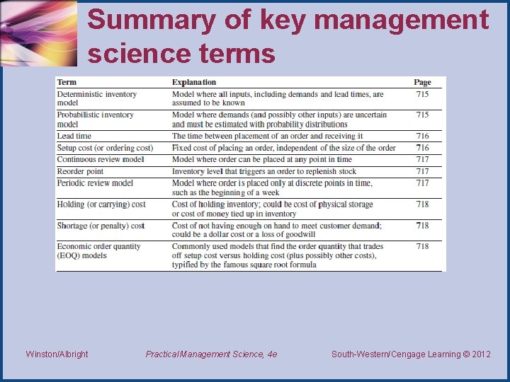
Summary of key management science terms Winston/Albright Practical Management Science, 4 e South-Western/Cengage Learning © 2012 Thomson/South-Western 2007 ©

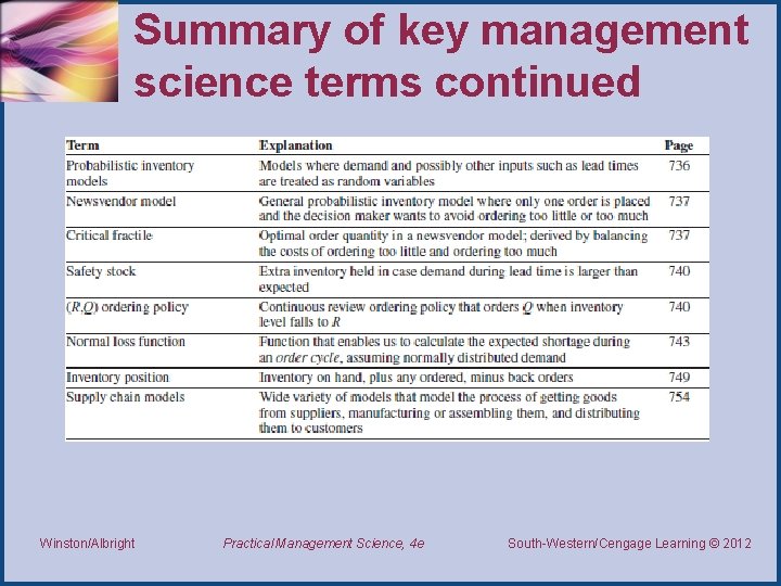
Summary of key management science terms continued Winston/Albright Practical Management Science, 4 e South-Western/Cengage Learning © 2012 Thomson/South-Western 2007 ©

End of Chapter 12