Chapter 12 Independent Demand Inventory Management Operations Management

Chapter 12 – Independent Demand Inventory Management Operations Management by R. Dan Reid & Nada R. Sanders 3 rd Edition © Wiley 2007

Inventory n n Independent demand: usually demand for finished goods that comes from outside customers—usually predicted from forecasts. Dependent demand: demand for raw materials, components, etc. needed to produce an item—usually calculated from the Master Production Schedule. (Chapter 15)

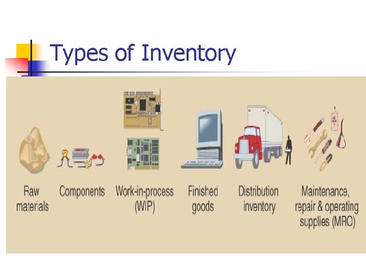
Types of Inventory

Uses of Inventory n n n Anticipation or seasonal inventory Safety stock: buffer demand fluctuations Lot-size or cycle stock: take advantage of quantity discounts or purchasing efficiencies Pipeline or transportation inventory Speculative or hedge inventory protects against some future event, e. g. labor strike Maintenance, repair, and operating (MRO) inventories

Decisions in Inventory Management n When to order or schedule a delivery? n How much to order or have delivered?

Inventory Management Objectives n Provide desired customer service level: n n n Provide for cost-efficient operations: n n Percentage of orders shipped on schedule Percentage of line items shipped on schedule Percentage of dollar volume shipped on schedule Idle time due to material and component shortages Buffer stock for smooth production flow Maintain a level work force Allowing longer production runs & quantity discounts Minimize inventory related investments: n n Inventory turnover Weeks (or days) of supply

Customer Service Level Examples n Percentage of Orders Shipped on Schedule n n n Percentage of Line Items Shipped on Schedule n n n Good measure if orders have similar value. Does not capture value. If one company represents 50% of your business but only 5% of your orders, 95% on schedule could represent only 50% of value Recognizes that not all orders are equal, but does not capture $ value of orders. More expensive to measure. Ok for finished goods. A 90% service level might mean shipping 225 items out of the total 250 line items totaled from 20 orders scheduled Percentage Of Dollar Volume Shipped on Schedule n Recognizes the differences in orders in terms of both line items and $ value

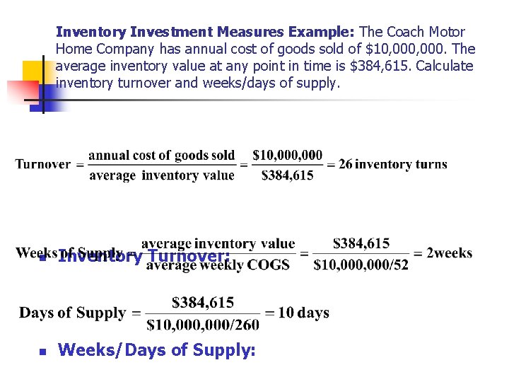
Inventory Investment Measures Example: The Coach Motor Home Company has annual cost of goods sold of $10, 000. The average inventory value at any point in time is $384, 615. Calculate inventory turnover and weeks/days of supply. n Inventory Turnover: n Weeks/Days of Supply:

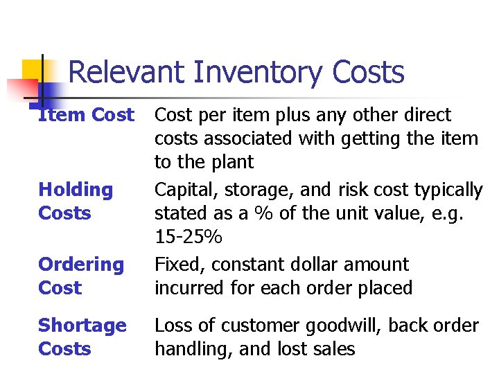
Relevant Inventory Costs Item Cost Ordering Cost per item plus any other direct costs associated with getting the item to the plant Capital, storage, and risk cost typically stated as a % of the unit value, e. g. 15 -25% Fixed, constant dollar amount incurred for each order placed Shortage Costs Loss of customer goodwill, back order handling, and lost sales Holding Costs

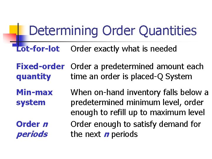
Determining Order Quantities Lot-for-lot Order exactly what is needed Fixed-order Order a predetermined amount each quantity time an order is placed-Q System Min-max system Order n periods When on-hand inventory falls below a predetermined minimum level, order enough to refill up to maximum level Order enough to satisfy demand for the next n periods

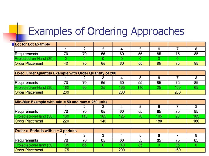
Examples of Ordering Approaches

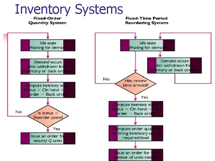
Inventory Systems

Reorder Point Systems n n Fixed reorder point and order quantity. Lead time—established reorder point. Two-bin system (manual system). Perpetual inventory system (usually a computerized, database system).

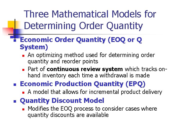
Three Mathematical Models for Determining Order Quantity n Economic Order Quantity (EOQ or Q System) n n n Economic Production Quantity (EPQ) n n An optimizing method used for determining order quantity and reorder points Part of continuous review system which tracks onhand inventory each time a withdrawal is made A model that allows for incremental product delivery Quantity Discount Model n Modifies the EOQ process to consider cases where quantity discounts are available

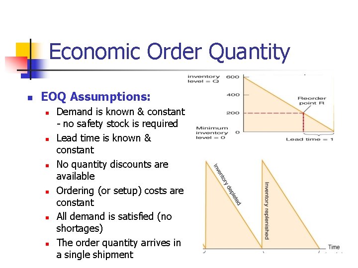
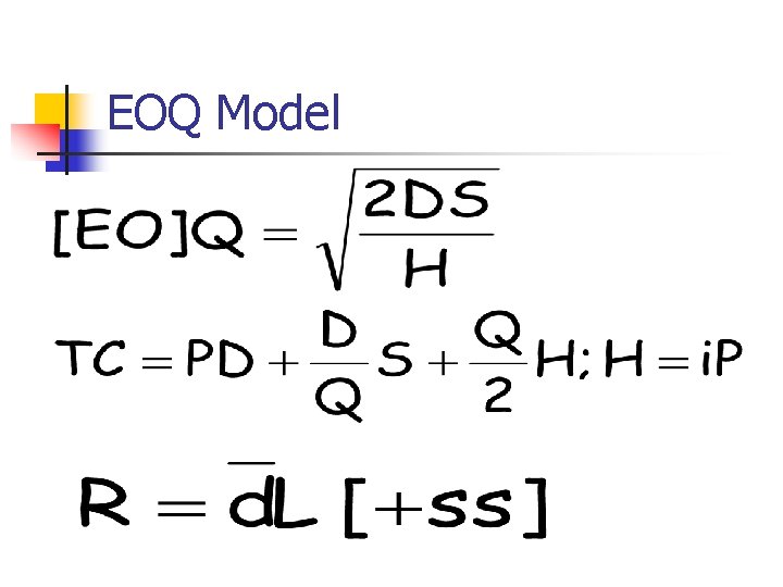
Economic Order Quantity n EOQ Assumptions: n n n Demand is known & constant - no safety stock is required Lead time is known & constant No quantity discounts are available Ordering (or setup) costs are constant All demand is satisfied (no shortages) The order quantity arrives in a single shipment

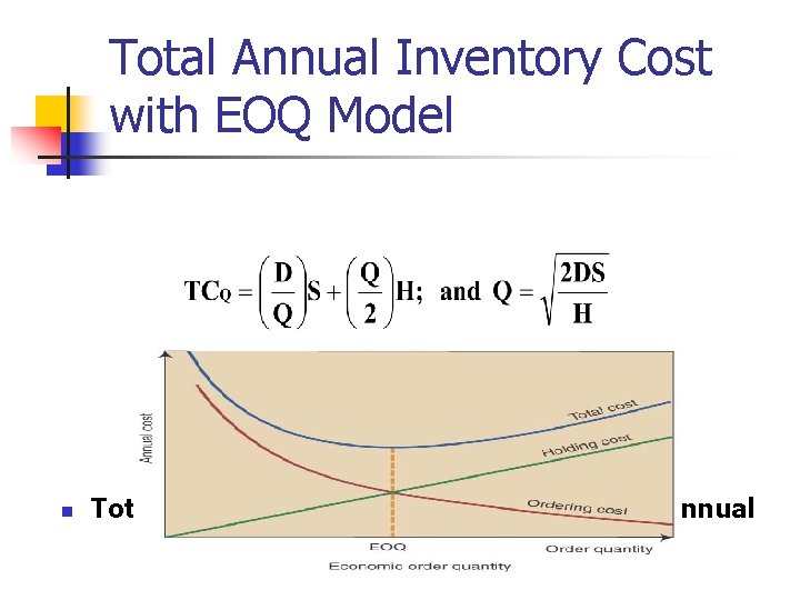
Total Annual Inventory Cost with EOQ Model n Total annual cost= annual ordering cost + annual holding costs

EOQ Model

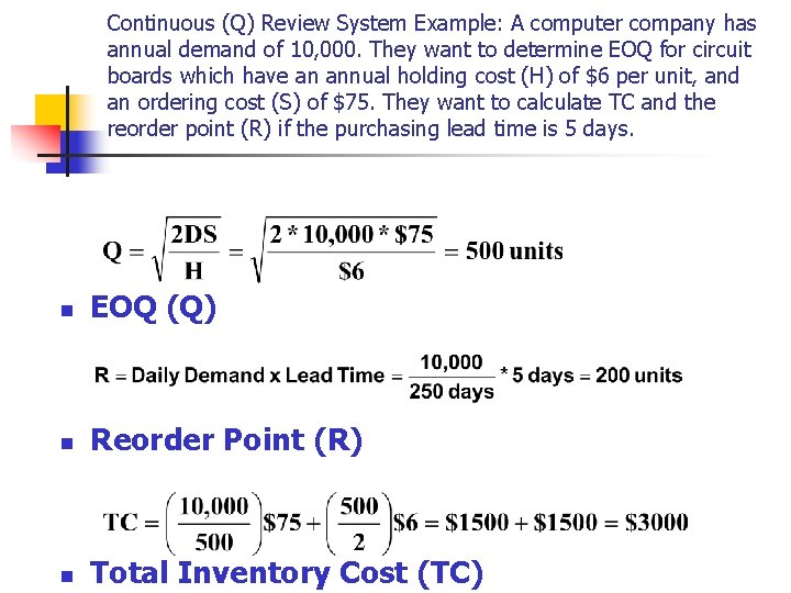
Continuous (Q) Review System Example: A computer company has annual demand of 10, 000. They want to determine EOQ for circuit boards which have an annual holding cost (H) of $6 per unit, and an ordering cost (S) of $75. They want to calculate TC and the reorder point (R) if the purchasing lead time is 5 days. n EOQ (Q) n Reorder Point (R) n Total Inventory Cost (TC)

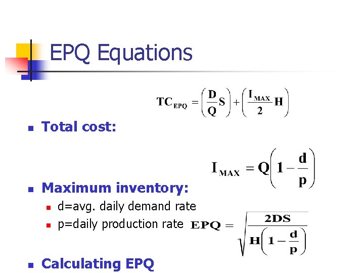
Fixed Order Quantity with Usage Model (EPQ) n n Model used when the stock (inventory) of an item is periodically being re-supplied concurrently with it being drawn from stock. The production rate must exceed the usage rate for this model to work. No homework or test problem will be based on this model

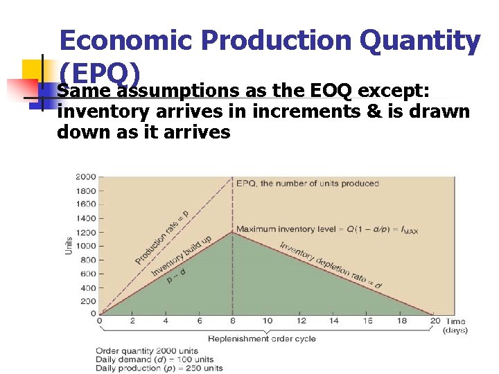
n Economic Production Quantity (EPQ) Same assumptions as the EOQ except: inventory arrives in increments & is drawn down as it arrives

EPQ Equations n Total cost: n Maximum inventory: n n n d=avg. daily demand rate p=daily production rate Calculating EPQ

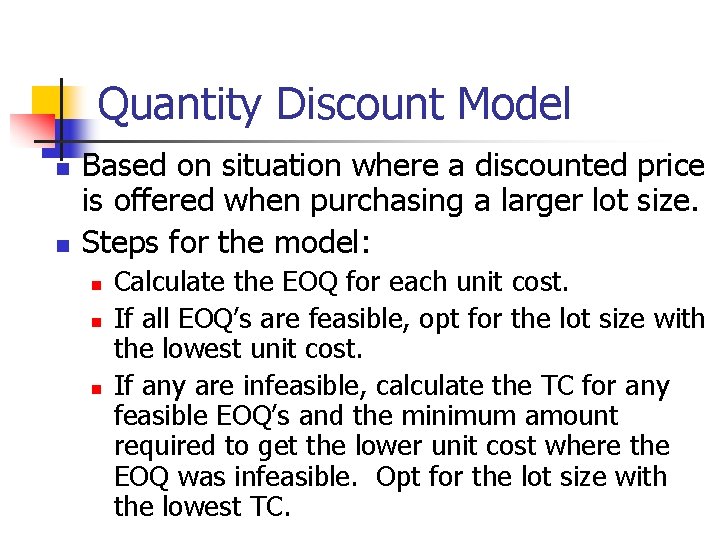
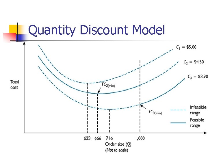
Quantity Discount Model n n Based on situation where a discounted price is offered when purchasing a larger lot size. Steps for the model: n n n Calculate the EOQ for each unit cost. If all EOQ’s are feasible, opt for the lot size with the lowest unit cost. If any are infeasible, calculate the TC for any feasible EOQ’s and the minimum amount required to get the lower unit cost where the EOQ was infeasible. Opt for the lot size with the lowest TC.

Quantity Discount Model

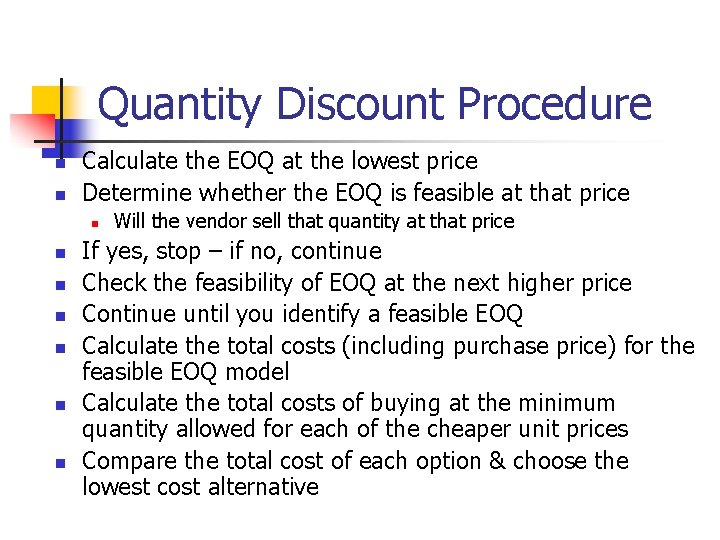
Quantity Discount Procedure n n Calculate the EOQ at the lowest price Determine whether the EOQ is feasible at that price n n n n Will the vendor sell that quantity at that price If yes, stop – if no, continue Check the feasibility of EOQ at the next higher price Continue until you identify a feasible EOQ Calculate the total costs (including purchase price) for the feasible EOQ model Calculate the total costs of buying at the minimum quantity allowed for each of the cheaper unit prices Compare the total cost of each option & choose the lowest cost alternative

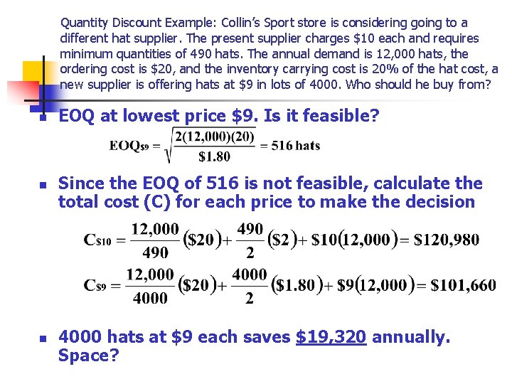
Quantity Discount Example: Collin’s Sport store is considering going to a different hat supplier. The present supplier charges $10 each and requires minimum quantities of 490 hats. The annual demand is 12, 000 hats, the ordering cost is $20, and the inventory carrying cost is 20% of the hat cost, a new supplier is offering hats at $9 in lots of 4000. Who should he buy from? n n n EOQ at lowest price $9. Is it feasible? Since the EOQ of 516 is not feasible, calculate the total cost (C) for each price to make the decision 4000 hats at $9 each saves $19, 320 annually. Space?

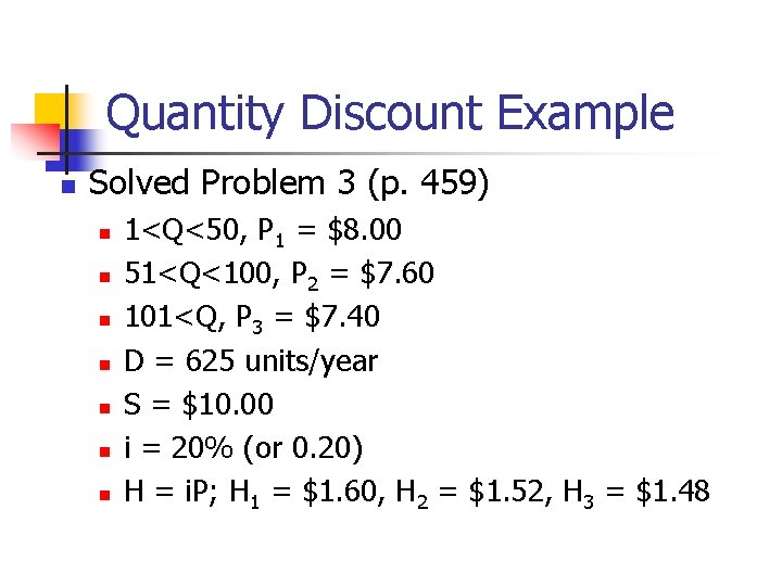
Quantity Discount Example n Solved Problem 3 (p. 459) n n n n 1<Q<50, P 1 = $8. 00 51<Q<100, P 2 = $7. 60 101<Q, P 3 = $7. 40 D = 625 units/year S = $10. 00 i = 20% (or 0. 20) H = i. P; H 1 = $1. 60, H 2 = $1. 52, H 3 = $1. 48

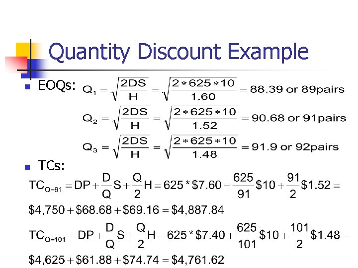
Quantity Discount Example n EOQs: n TCs:

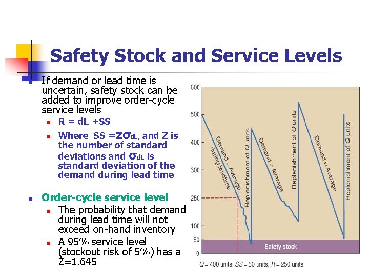
Safety Stock and Service Levels n If demand or lead time is uncertain, safety stock can be added to improve order-cycle service levels n n n R = d. L +SS Where SS =zσd. L, and Z is the number of standard deviations and σd. L is standard deviation of the demand during lead time Order-cycle service level n The probability that demand during lead time will not exceed on-hand inventory n A 95% service level (stockout risk of 5%) has a Z=1. 645

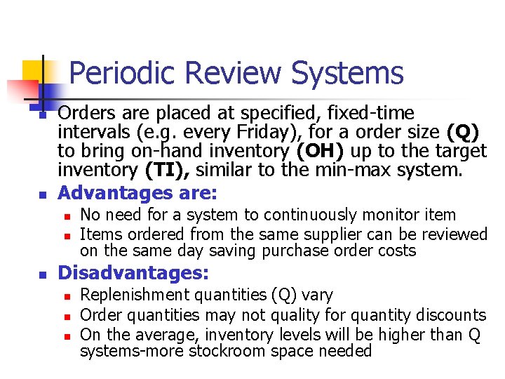
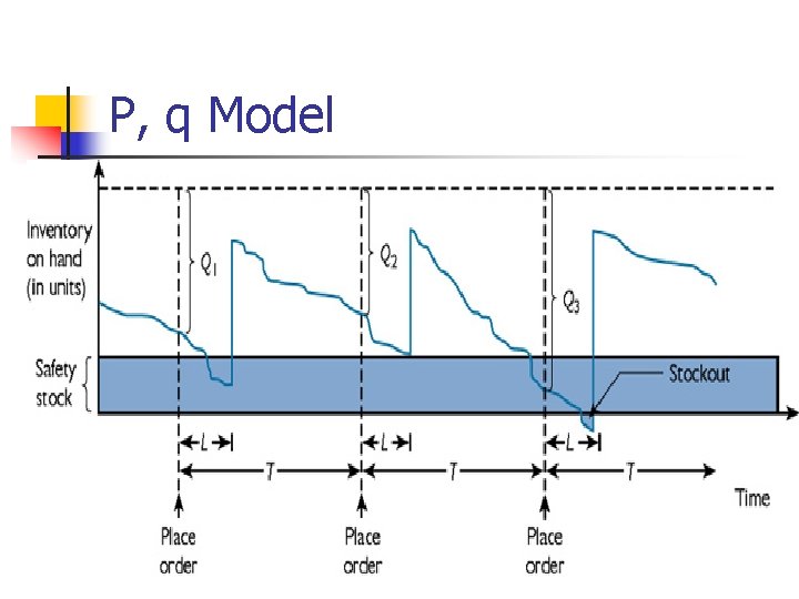
Periodic Review Systems n n Orders are placed at specified, fixed-time intervals (e. g. every Friday), for a order size (Q) to bring on-hand inventory (OH) up to the target inventory (TI), similar to the min-max system. Advantages are: n n n No need for a system to continuously monitor item Items ordered from the same supplier can be reviewed on the same day saving purchase order costs Disadvantages: n n n Replenishment quantities (Q) vary Order quantities may not quality for quantity discounts On the average, inventory levels will be higher than Q systems-more stockroom space needed

P, q Model

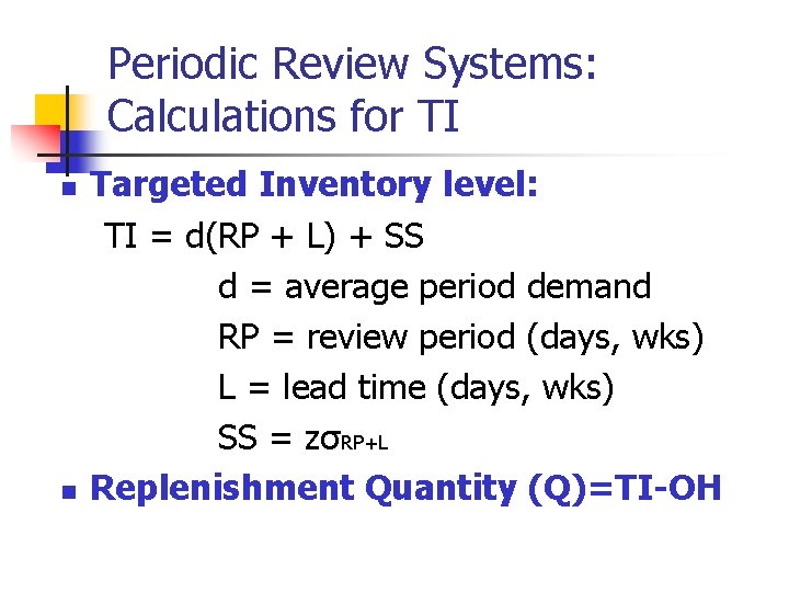
Periodic Review Systems: Calculations for TI n n Targeted Inventory level: TI = d(RP + L) + SS d = average period demand RP = review period (days, wks) L = lead time (days, wks) SS = zσRP+L Replenishment Quantity (Q)=TI-OH

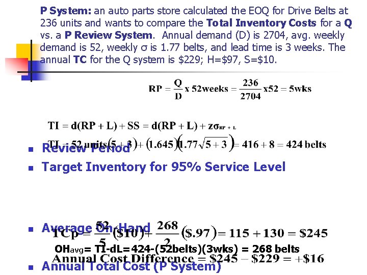
P System: an auto parts store calculated the EOQ for Drive Belts at 236 units and wants to compare the Total Inventory Costs for a Q vs. a P Review System. Annual demand (D) is 2704, avg. weekly demand is 52, weekly σ is 1. 77 belts, and lead time is 3 weeks. The annual TC for the Q system is $229; H=$97, S=$10. n Review Period n Target Inventory for 95% Service Level n Average On-Hand OHavg= TI-d. L=424 -(52 belts)(3 wks) = 268 belts n Annual Total Cost (P System)

Single Period Inventory Model n The SPI model is designed for products that share the following characteristics: n n Sold at their regular price only during a single-time period Demand is highly variable but follows a known probability distribution Salvage value is less than its original cost so money is lost when these products are sold for their salvage value Objective is to balance the gross profit of the sale of a unit with the cost incurred when a unit is sold after its primary selling period

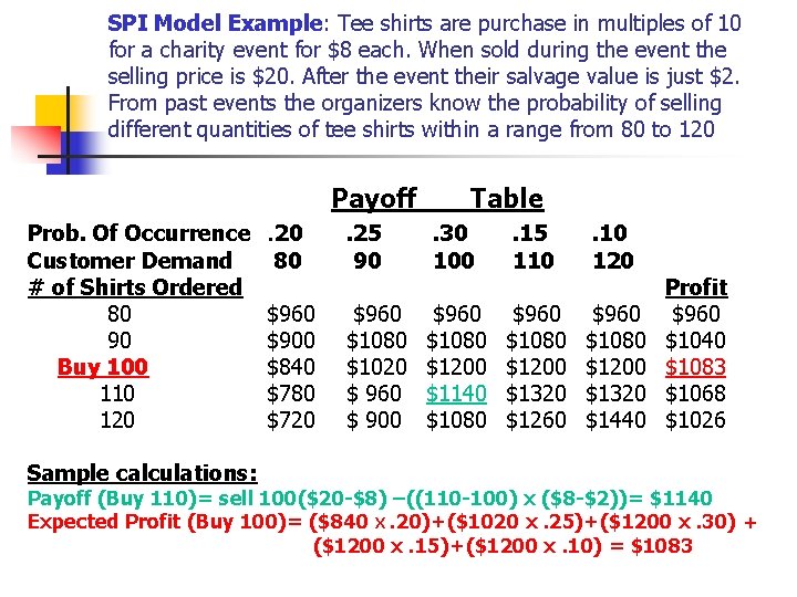
SPI Model Example: Tee shirts are purchase in multiples of 10 for a charity event for $8 each. When sold during the event the selling price is $20. After the event their salvage value is just $2. From past events the organizers know the probability of selling different quantities of tee shirts within a range from 80 to 120 Payoff Prob. Of Occurrence Customer Demand # of Shirts Ordered 80 90 Buy 100 110 120 Sample calculations: . 20 80 $960 $900 $840 $780 $720 Table . 25 90 . 30 100 . 15 110 . 10 120 $960 $1080 $1020 $ 960 $ 900 $960 $1080 $1200 $1140 $1080 $960 $1080 $1200 $1320 $1260 $960 $1080 $1200 $1320 $1440 Profit $960 $1040 $1083 $1068 $1026 Payoff (Buy 110)= sell 100($20 -$8) –((110 -100) x ($8 -$2))= $1140 Expected Profit (Buy 100)= ($840 X. 20)+($1020 x. 25)+($1200 x. 30) + ($1200 x. 15)+($1200 x. 10) = $1083

Yield (or Revenue) Management n n Concept similar to single-period inventory model—but the issue is not with inventory, but with maximizing the utilization of available capacity which cannot be carried over as stock. Decisions often consider allocating amounts of capacity to differing price levels. The goal is make an allocation that will maximize revenue.

ABC Classification n Divide inventories into A, B, and C categories based on value, risk, & other considerations n n n Use tight controls & frequent reviews for A items Use normal methods to manage B items Use simple, inexpensive systems with large safety stocks to manage C items (just don’t run out)

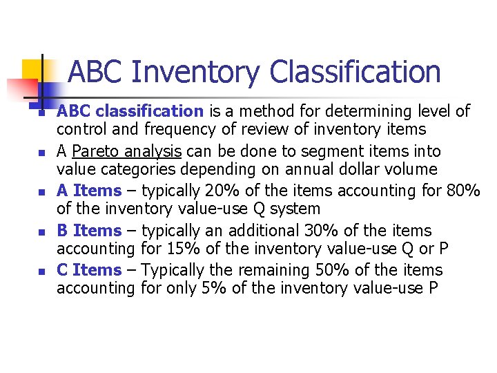
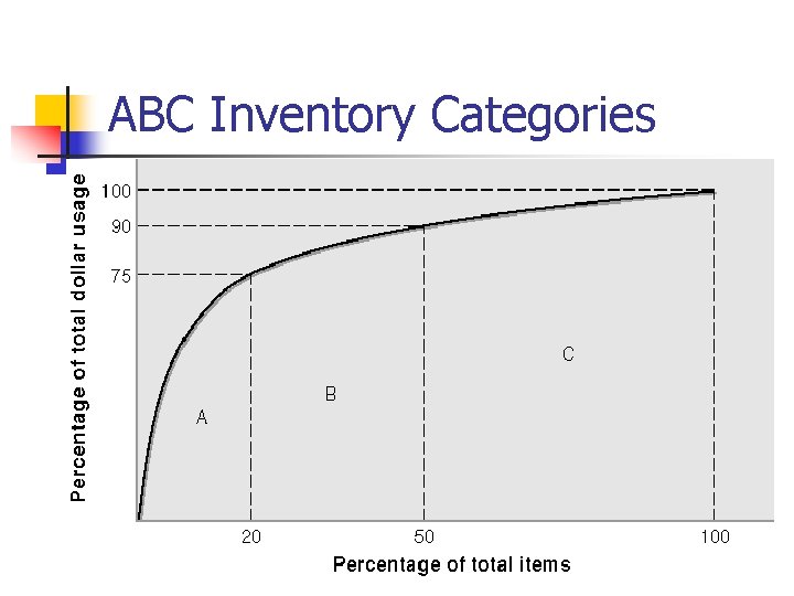
ABC Inventory Classification n n ABC classification is a method for determining level of control and frequency of review of inventory items A Pareto analysis can be done to segment items into value categories depending on annual dollar volume A Items – typically 20% of the items accounting for 80% of the inventory value-use Q system B Items – typically an additional 30% of the items accounting for 15% of the inventory value-use Q or P C Items – Typically the remaining 50% of the items accounting for only 5% of the inventory value-use P

ABC Inventory Categories

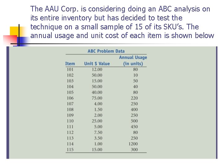
The AAU Corp. is considering doing an ABC analysis on its entire inventory but has decided to test the technique on a small sample of 15 of its SKU’s. The annual usage and unit cost of each item is shown below

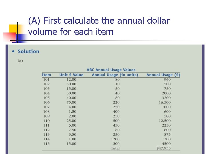
(A) First calculate the annual dollar volume for each item

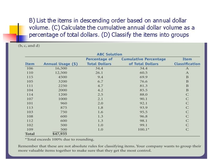
B) List the items in descending order based on annual dollar volume. (C) Calculate the cumulative annual dollar volume as a percentage of total dollars. (D) Classify the items into groups

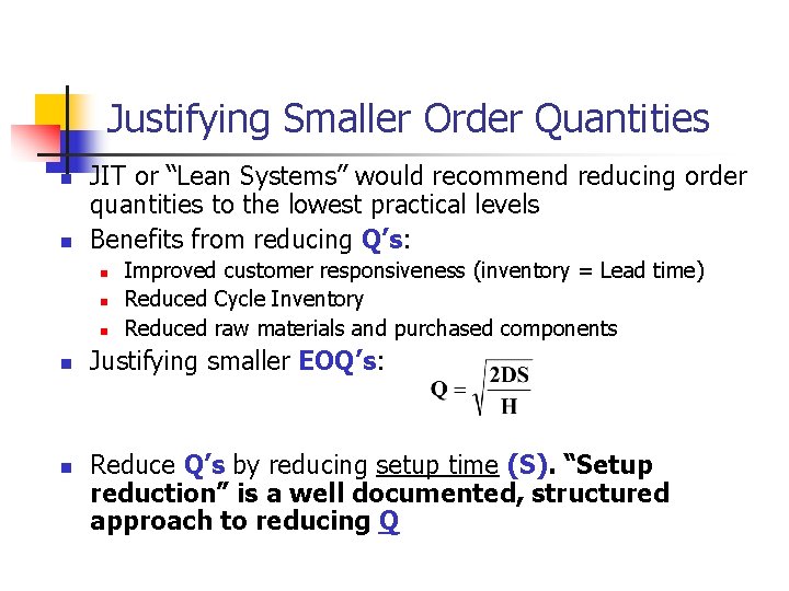
Justifying Smaller Order Quantities n n JIT or “Lean Systems” would recommend reducing order quantities to the lowest practical levels Benefits from reducing Q’s: n n n Improved customer responsiveness (inventory = Lead time) Reduced Cycle Inventory Reduced raw materials and purchased components Justifying smaller EOQ’s: Reduce Q’s by reducing setup time (S). “Setup reduction” is a well documented, structured approach to reducing Q

Inventory Record Accuracy n Inaccurate inventory records can cause: n n n Lost sales Disrupted operations Poor customer service Lower productivity Planning errors and expediting Two methods are available for checking record accuracy n n Periodic counting-usually an annual physical inventory to verify and update records Cycle counting-daily counting of pre-specified items (often using ABC classification) provides the following advantages: n n n Timely detection and correction of inaccurate records Elimination of lost production time due to unexpected stock outs Structured approach using employees trained in cycle counting

Inventory Management Across the Organization n Inventory management policies affect functional areas throughout n n n Accounting is concerned of the cost implications of inventory Marketing is concerned as stocking decision affect the level of customer service Information Systems is involved to tack and control inventory records

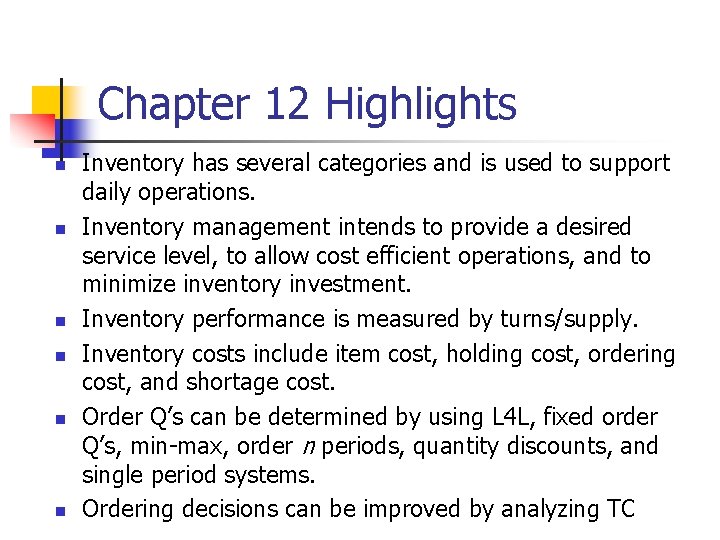
Chapter 12 Highlights n n n Inventory has several categories and is used to support daily operations. Inventory management intends to provide a desired service level, to allow cost efficient operations, and to minimize inventory investment. Inventory performance is measured by turns/supply. Inventory costs include item cost, holding cost, ordering cost, and shortage cost. Order Q’s can be determined by using L 4 L, fixed order Q’s, min-max, order n periods, quantity discounts, and single period systems. Ordering decisions can be improved by analyzing TC

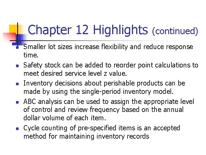
Chapter 12 Highlights n n n (continued) Smaller lot sizes increase flexibility and reduce response time. Safety stock can be added to reorder point calculations to meet desired service level z value. Inventory decisions about perishable products can be made by using the single-period inventory model. ABC analysis can be used to assign the appropriate level of control and review frequency based on the annual dollar volume of each item. Cycle counting of pre-specified items is an accepted method for maintaining inventory records

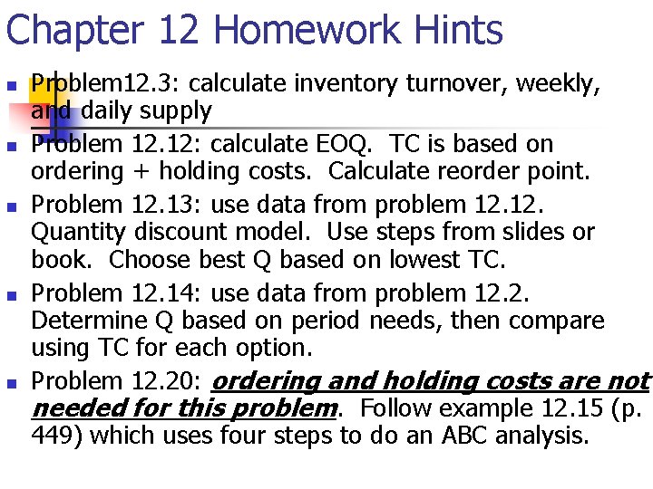
Chapter 12 Homework Hints n n n Problem 12. 3: calculate inventory turnover, weekly, and daily supply Problem 12. 12: calculate EOQ. TC is based on ordering + holding costs. Calculate reorder point. Problem 12. 13: use data from problem 12. Quantity discount model. Use steps from slides or book. Choose best Q based on lowest TC. Problem 12. 14: use data from problem 12. 2. Determine Q based on period needs, then compare using TC for each option. Problem 12. 20: ordering and holding costs are not needed for this problem. Follow example 12. 15 (p. 449) which uses four steps to do an ABC analysis.