Introduction to Matrices Douglas N Greve grevenmr mgh

Introduction to Matrices Douglas N. Greve greve@nmr. mgh. harvard. edu

Why Matrices? • Simplifies notation • Simplifies concepts • Grounding for general linear model (GLM) • Simplifies implementation (eg, matlab, octave) • Optimization

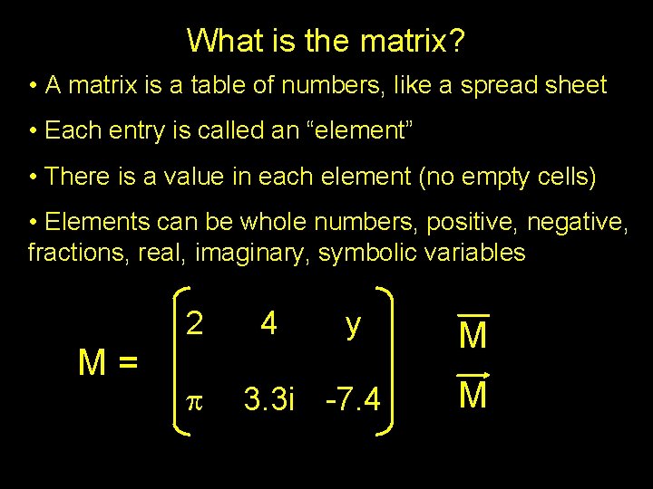
What is the matrix? • A matrix is a table of numbers, like a spread sheet • Each entry is called an “element” • There is a value in each element (no empty cells) • Elements can be whole numbers, positive, negative, fractions, real, imaginary, symbolic variables 2 M= p 4 y 3. 3 i -7. 4 M M

Parts of Matrices • Size/Dimensions • Elements • Groupings of Elements • Diagonals • Triangles • Vectors

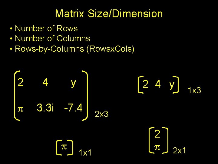
Matrix Size/Dimension • Number of Rows • Number of Columns • Rows-by-Columns (Rowsx. Cols) 2 p 4 y 2 4 y 3. 3 i -7. 4 p 1 x 1 2 x 3 2 p 2 x 1 1 x 3

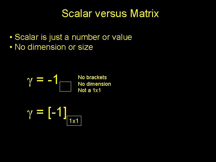
Scalar versus Matrix • Scalar is just a number or value • No dimension or size g = -1 No brackets No dimension Not a 1 x 1 g = [-1] 1 x 1

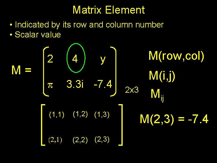
Matrix Element • Indicated by its row and column number • Scalar value M= 2 p 4 M(row, col) y 3. 3 i -7. 4 (1, 1) (1, 2) (1, 3) (2, 1) (2, 2) (2, 3) M(i, j) 2 x 3 Mij M(2, 3) = -7. 4

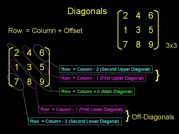
Diagonals Row = Column + Offset 7 8 9 1 3 5 7 8 9 2 4 6 1 3 5 2 4 6 Row = Column - 2 (Second Upper Diagonal) Row = Column - 1 (First Upper Diagonal) 3 x 3 } Row = Column + 0 (Main Diagonal) Row = Column - 1 (First Lower Diagonal) Row = Column - 2 (Second Lower Diagonal) } Off-Diagonals

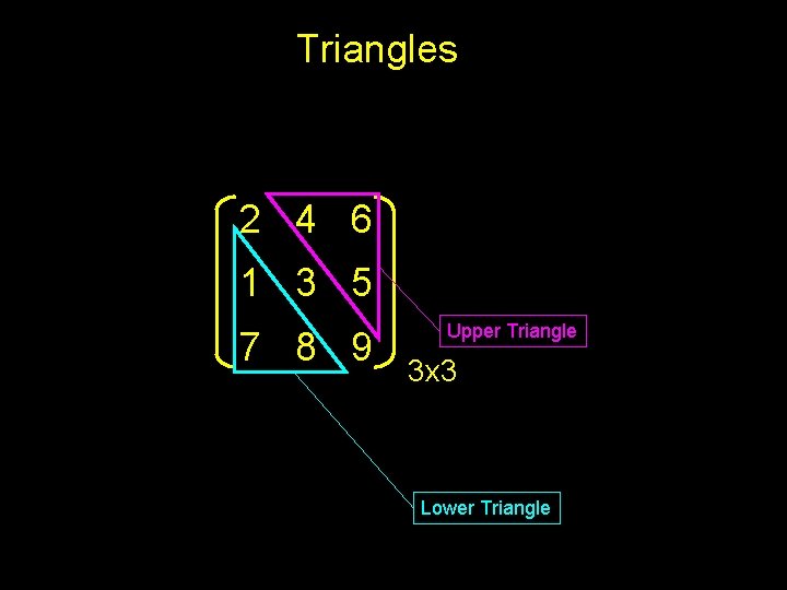
Triangles 2 4 6 1 3 5 7 8 9 Upper Triangle 3 x 3 Lower Triangle

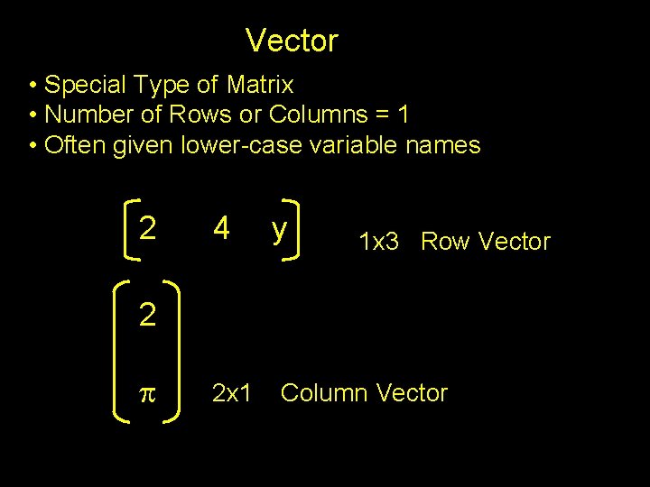
Vector • Special Type of Matrix • Number of Rows or Columns = 1 • Often given lower-case variable names 2 4 y 1 x 3 Row Vector 2 p 2 x 1 Column Vector

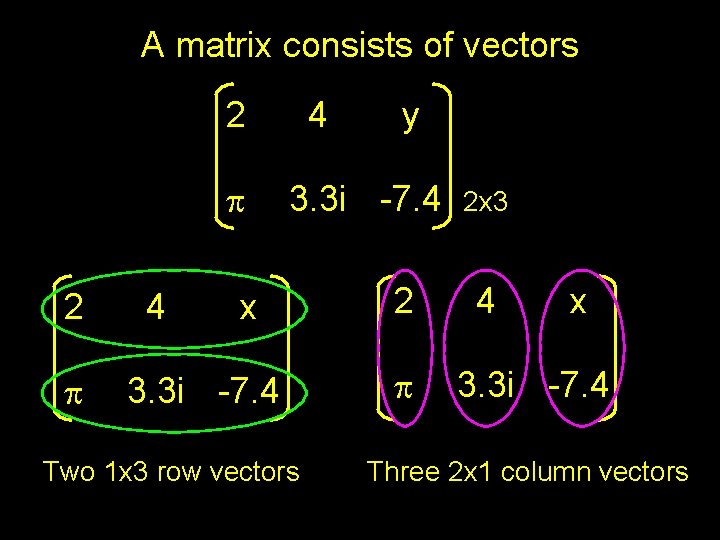
A matrix consists of vectors 2 p 4 4 y 3. 3 i -7. 4 x 3. 3 i -7. 4 Two 1 x 3 row vectors 2 p 2 x 3 4 x 3. 3 i -7. 4 Three 2 x 1 column vectors

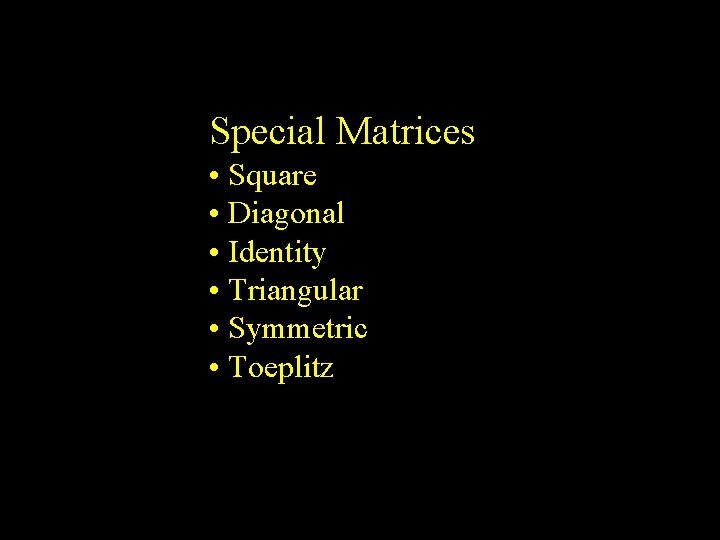
Special Matrices • Square • Diagonal • Identity • Triangular • Symmetric • Toeplitz

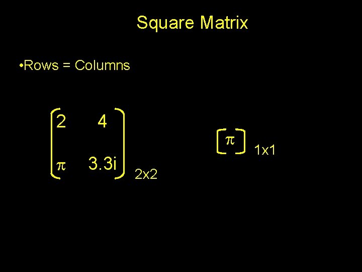
Square Matrix • Rows = Columns 2 p 4 3. 3 i p 2 x 2 1 x 1

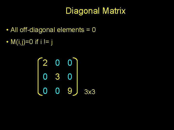
Diagonal Matrix • All off-diagonal elements = 0 • M(i, j)=0 if i != j 2 0 0 0 3 0 0 0 9 3 x 3

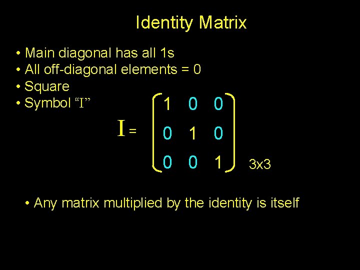
Identity Matrix • Main diagonal has all 1 s • All off-diagonal elements = 0 • Square • Symbol “I” 1 0 I= 0 0 1 0 0 0 1 3 x 3 • Any matrix multiplied by the identity is itself

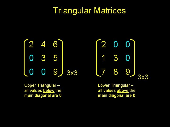
Triangular Matrices 2 4 6 2 0 0 0 3 5 1 3 0 0 0 9 Upper Triangular – all values below the main diagonal are 0 3 x 3 7 8 9 Lower Triangular – all values above the main diagonal are 0 3 x 3

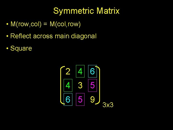
Symmetric Matrix • M(row, col) = M(col, row) • Reflect across main diagonal • Square 2 4 6 4 3 5 6 5 9 3 x 3

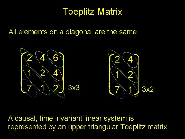
Toeplitz Matrix All elements on a diagonal are the same 2 4 6 2 4 1 2 7 1 2 3 x 3 7 1 3 x 2 A causal, time invariant linear system is represented by an upper triangular Toeplitz matrix

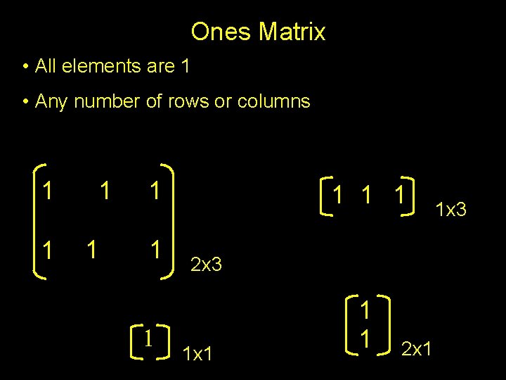
Ones Matrix • All elements are 1 • Any number of rows or columns 1 1 1 1 1 2 x 3 1 x 1 1 1 2 x 1 1 x 3

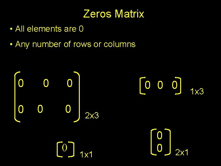
Zeros Matrix • All elements are 0 • Any number of rows or columns 0 0 0 0 0 2 x 3 1 x 1 0 0 2 x 1 1 x 3

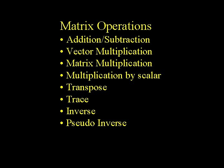
Matrix Operations • Addition/Subtraction • Vector Multiplication • Matrix Multiplication • Multiplication by scalar • Transpose • Trace • Inverse • Pseudo Inverse

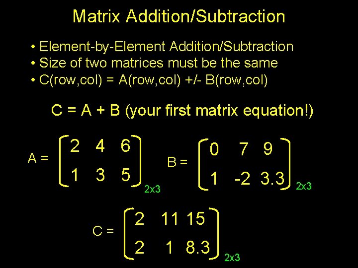
Matrix Addition/Subtraction • Element-by-Element Addition/Subtraction • Size of two matrices must be the same • C(row, col) = A(row, col) +/- B(row, col) C = A + B (your first matrix equation!) A= 2 4 6 1 3 5 C= B= 2 x 3 0 7 9 1 -2 3. 3 2 11 15 2 1 8. 3 2 x 3

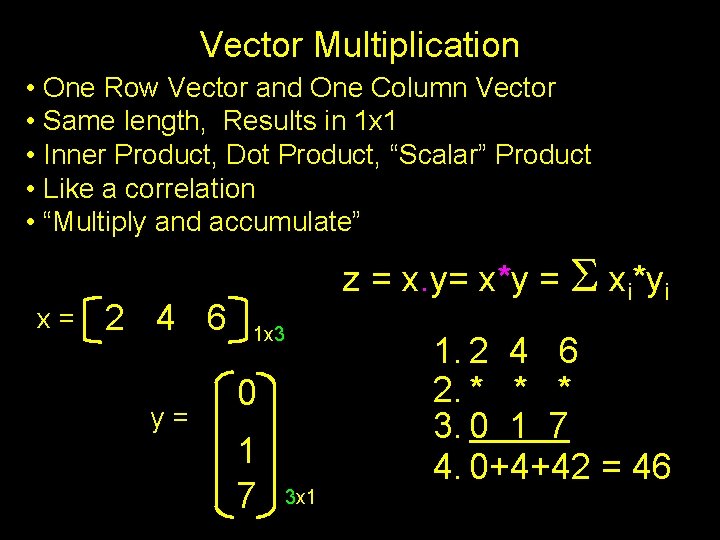
Vector Multiplication • One Row Vector and One Column Vector • Same length, Results in 1 x 1 • Inner Product, Dot Product, “Scalar” Product • Like a correlation • “Multiply and accumulate” x= 2 4 6 y= z = x. y= x*y = S xi*yi 1 x 3 0 1 7 3 x 1 1. 2 4 6 2. * * * 3. 0 1 7 4. 0+4+42 = 46

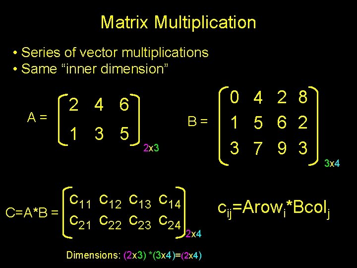
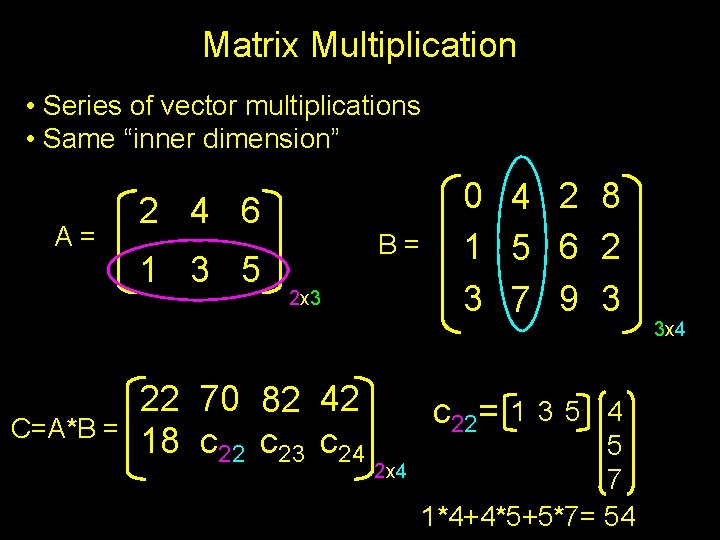
Matrix Multiplication • Series of vector multiplications • Same “inner dimension” A= C=A*B = 2 4 6 1 3 5 B= 2 x 3 c 11 c 12 c 13 c 14 c 21 c 22 c 23 c 24 0 4 2 8 1 5 6 2 3 7 9 3 3 x 4 cij=Arowi*Bcolj 2 x 4 Dimensions: (2 x 3) *(3 x 4)=(2 x 4)

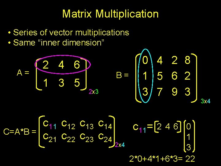
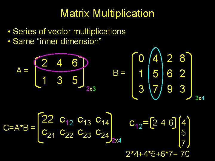
Matrix Multiplication • Series of vector multiplications • Same “inner dimension” A= C=A*B = 2 4 6 1 3 5 B= 2 x 3 c 11 c 12 c 13 c 14 c 21 c 22 c 23 c 24 0 4 2 8 1 5 6 2 3 7 9 3 c 11= 2 x 4 2 4 6 0 1 3 2*0+4*1+6*3= 22 3 x 4

Matrix Multiplication • Series of vector multiplications • Same “inner dimension” A= C=A*B = 2 4 6 1 3 5 B= 2 x 3 22 c 13 c 14 c 21 c 22 c 23 c 24 0 4 2 8 1 5 6 2 3 7 9 3 c 12= 2 x 4 2 4 6 4 5 7 2*4+4*5+6*7= 70 3 x 4

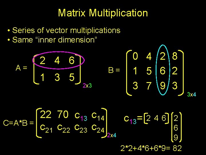
Matrix Multiplication • Series of vector multiplications • Same “inner dimension” A= C=A*B = 2 4 6 1 3 5 B= 2 x 3 22 70 c 13 c 14 c 21 c 22 c 23 c 24 0 4 2 8 1 5 6 2 3 7 9 3 c 13= 2 x 4 2 4 6 2 6 9 2*2+4*6+6*9= 82 3 x 4

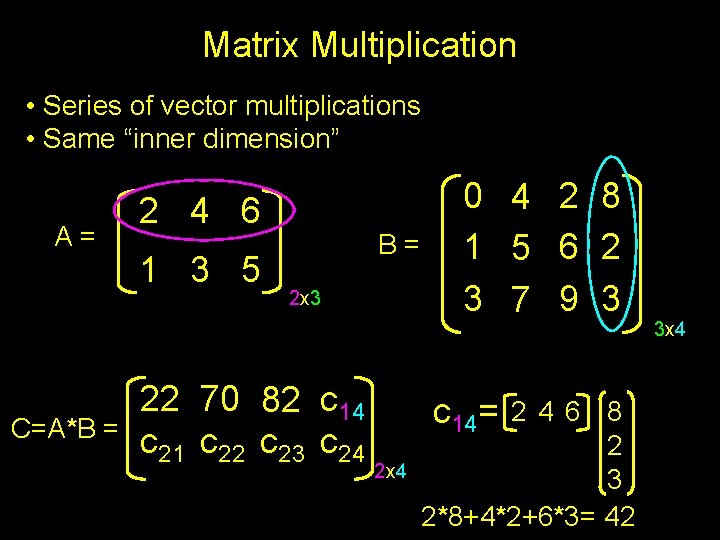
Matrix Multiplication • Series of vector multiplications • Same “inner dimension” A= C=A*B = 2 4 6 1 3 5 B= 2 x 3 22 70 82 c 14 c 21 c 22 c 23 c 24 0 4 2 8 1 5 6 2 3 7 9 3 c 14= 2 x 4 2 4 6 8 2 3 2*8+4*2+6*3= 42 3 x 4

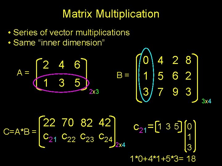
Matrix Multiplication • Series of vector multiplications • Same “inner dimension” A= C=A*B = 2 4 6 1 3 5 B= 2 x 3 22 70 82 42 c 21 c 22 c 23 c 24 0 4 2 8 1 5 6 2 3 7 9 3 c 21= 2 x 4 1 3 5 0 1 3 1*0+4*1+5*3= 18 3 x 4

Matrix Multiplication • Series of vector multiplications • Same “inner dimension” A= C=A*B = 2 4 6 1 3 5 B= 2 x 3 22 70 82 42 18 c 22 c 23 c 24 0 4 2 8 1 5 6 2 3 7 9 3 c 22= 2 x 4 1 3 5 4 5 7 1*4+4*5+5*7= 54 3 x 4

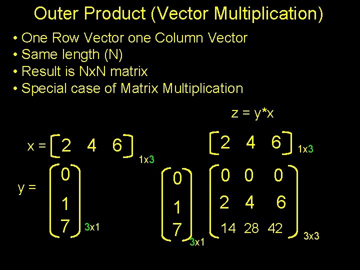
Outer Product (Vector Multiplication) • One Row Vector one Column Vector • Same length (N) • Result is Nx. N matrix • Special case of Matrix Multiplication z = y*x x= y= 2 4 6 0 1 7 2 4 6 1 x 3 0 0 2 4 0 3 x 1 1 7 0 6 14 28 42 3 x 1 1 x 3 3 x 3

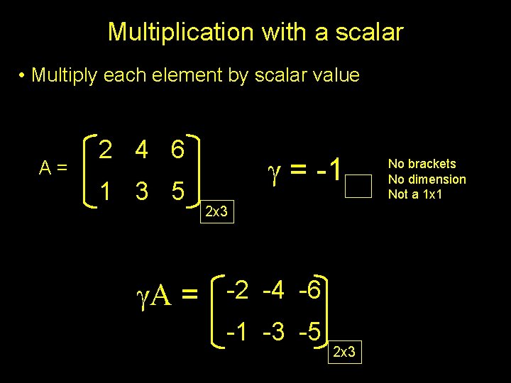
Multiplication with a scalar • Multiply each element by scalar value A= 2 4 6 1 3 5 g = -1 2 x 3 g. A = -2 -4 -6 -1 -3 -5 2 x 3 No brackets No dimension Not a 1 x 1

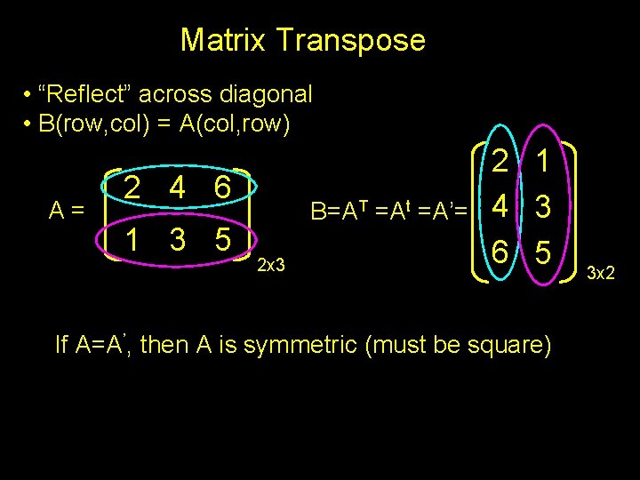
Matrix Transpose • “Reflect” across diagonal • B(row, col) = A(col, row) A= 2 4 6 1 3 5 B=AT =At =A’= 2 x 3 2 1 4 3 6 5 If A=A’, then A is symmetric (must be square) 3 x 2

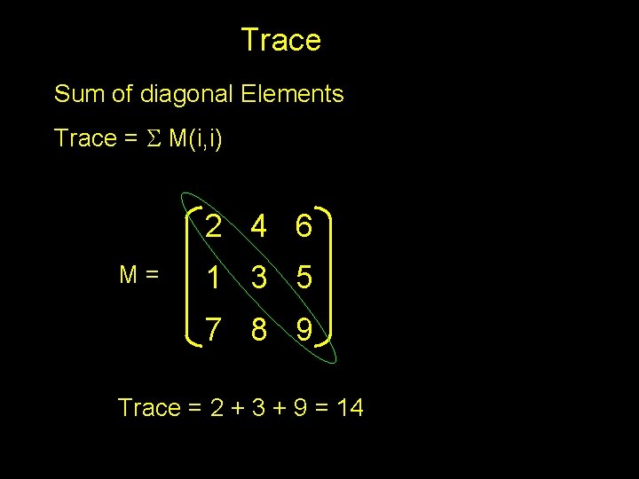
Trace Sum of diagonal Elements Trace = S M(i, i) 2 4 6 M= 1 3 5 7 8 9 Trace = 2 + 3 + 9 = 14

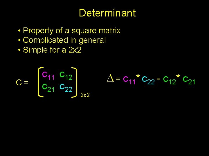
Determinant • Property of a square matrix • Complicated in general • Simple for a 2 x 2 C= c 11 c 12 c 21 c 22 D = c 11* c 22 - c 12* c 21 2 x 2

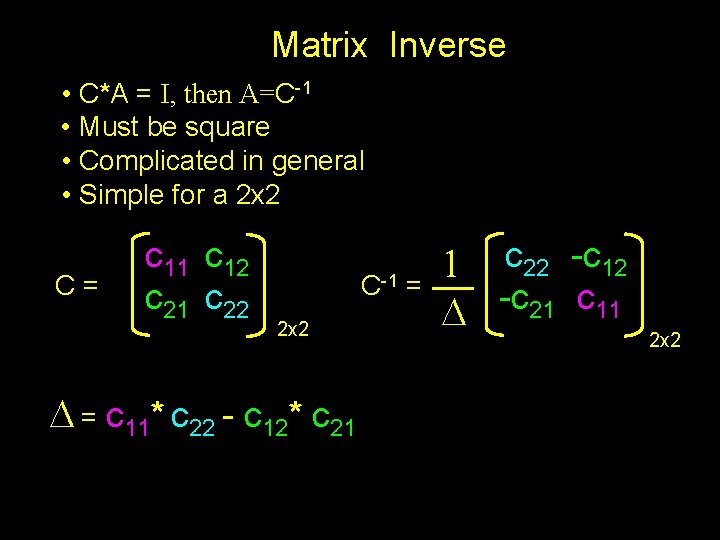
Matrix Inverse • C*A = I, then A=C-1 • Must be square • Complicated in general • Simple for a 2 x 2 C= c 11 c 12 c 21 c 22 C-1 = 2 x 2 D = c 11* c 22 - c 12* c 21 1 c 22 -c 12 -c c 21 11 D 2 x 2

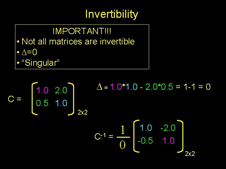
Invertibility IMPORTANT!!! • Not all matrices are invertible • D=0 • “Singular” C= D = 1. 0*1. 0 - 2. 0*0. 5 = 1 -1 = 0 1. 0 2. 0 0. 5 1. 0 2 x 2 C-1 = 1 0 1. 0 -2. 0 -0. 5 1. 0 2 x 2

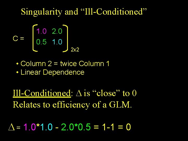
Singularity and “Ill-Conditioned” C= 1. 0 2. 0 0. 5 1. 0 2 x 2 • Column 2 = twice Column 1 • Linear Dependence Ill-Conditioned: D is “close” to 0 Relates to efficiency of a GLM. D = 1. 0*1. 0 - 2. 0*0. 5 = 1 -1 = 0

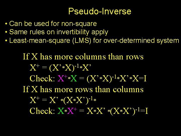
Pseudo-Inverse • Can be used for non-square • Same rules on invertibility apply • Least-mean-square (LMS) for over-determined system If X has more columns than rows X+ = (X’*X)-1*X’ Check: X+*X = (X’*X)-1*X’*X=I If X has more rows than columns X+ = X’ *(X*X’)-1* Check: X*X+ = X*X’ *(X*X’)-1=I

Matrix Applications

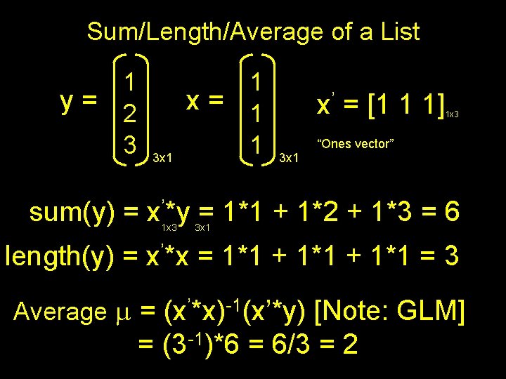
Sum/Length/Average of a List 1 y= 2 3 3 x 1 1 x= 1 1 x’ = [1 1 1] 1 x 3 “Ones vector” 3 x 1 sum(y) = x’*y = 1*1 + 1*2 + 1*3 = 6 1 x 3 3 x 1 length(y) = x’*x = 1*1 + 1*1 = 3 Average m = (x’*x)-1(x’*y) [Note: GLM] = (3 -1)*6 = 6/3 = 2

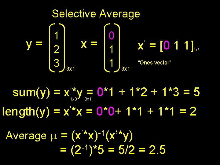
Selective Average 1 y= 2 3 3 x 1 0 x= 1 1 x’ = [0 1 1] 1 x 3 “Ones vector” 3 x 1 sum(y) = x’*y = 0*1 + 1*2 + 1*3 = 5 1 x 3 3 x 1 length(y) = x’*x = 0*0+ 1*1 = 2 Average m = (x’*x)-1(x’*y) = (2 -1)*5 = 5/2 = 2. 5

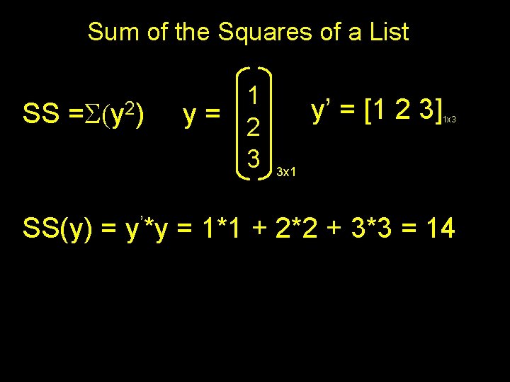
Sum of the Squares of a List SS =S(y 2) 1 y= 2 3 y’ = [1 2 3] 1 x 3 3 x 1 SS(y) = y’*y = 1*1 + 2*2 + 3*3 = 14

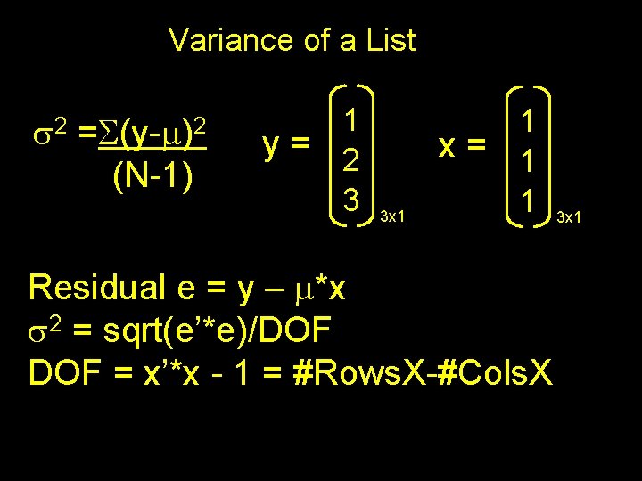
Variance of a List s 2 =S(y-m)2 (N-1) 1 y= 2 3 3 x 1 1 x= 1 1 Residual e = y – m*x s 2 = sqrt(e’*e)/DOF = x’*x - 1 = #Rows. X-#Cols. X 3 x 1

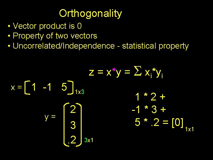
Orthogonality • Vector product is 0 • Property of two vectors • Uncorrelated/Independence - statistical property z = x*y = S xi*yi x= 1 -1 5 y= 1 x 3 2 3 x 1 1*2+ -1 * 3 + 5 *. 2 = [0] 1 x 1

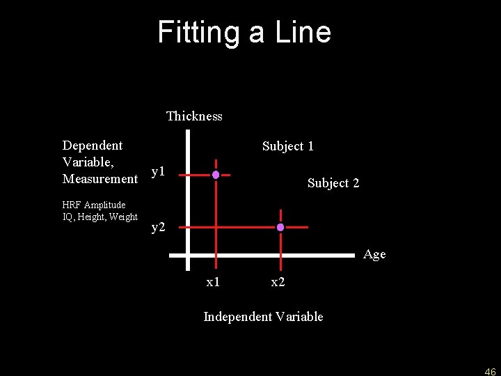
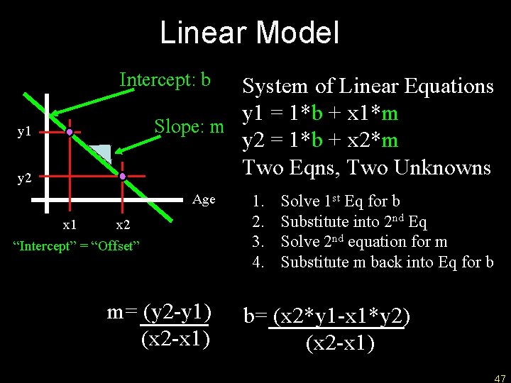
Fitting a Line Thickness Dependent Variable, y 1 Measurement HRF Amplitude IQ, Height, Weight Subject 1 Subject 2 y 2 Age x 1 x 2 Independent Variable 46

Linear Model Intercept: b System of Linear Equations y 1 = 1*b + x 1*m Slope: m y 2 = 1*b + x 2*m Two Eqns, Two Unknowns y 1 y 2 Age x 1 x 2 “Intercept” = “Offset” m= (y 2 -y 1) (x 2 -x 1) 1. 2. 3. 4. Solve 1 st Eq for b Substitute into 2 nd Eq Solve 2 nd equation for m Substitute m back into Eq for b b= (x 2*y 1 -x 1*y 2) (x 2 -x 1) 47

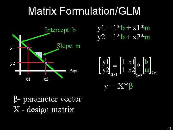
Matrix Formulation/GLM Intercept: b y 1 = 1*b + x 1*m y 2 = 1*b + x 2*m Slope: m y 1 y 2 Age x 1 x 2 y 1 1 x 1 b = 1 x 2 * m y 2 2 x 1 2 x 2 y = X*b b- parameter vector X - design matrix 48

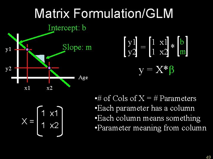
Matrix Formulation/GLM Intercept: b Slope: m y 1 y 2 Age x 1 y 1 1 x 1 b = * y 2 1 x 2 m y = X*b x 2 1 x 1 X = 1 x 2 • # of Cols of X = # Parameters • Each parameter has a column • Each column means something • Parameter meaning from column 49

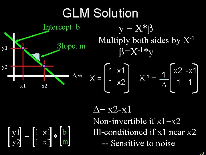
GLM Solution Intercept: b Slope: m y 1 y 2 Age x 1 x 2 y = X*b Multiply both sides by X-1 b=X-1*y 1 x 1 X = 1 x 2 -x 1 X-1 = 1 D -1 1 D= x 2 -x 1 y 1 1 x 1 b = 1 x 2 * m y 2 Non-invertible if x 1=x 2 Ill-conditioned if x 1 near x 2 -- Sensitive to noise 50

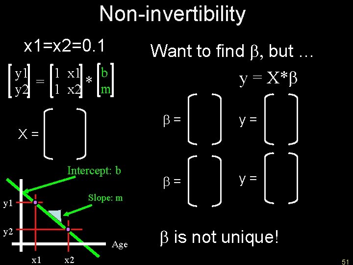
Non-invertibility x 1=x 2=0. 1 Want to find b, but … y 1 1 x 1 b = 1 x 2 * m y 2 X= Intercept: b y = X*b b= y= Slope: m y 1 y 2 Age x 1 x 2 b is not unique! 51

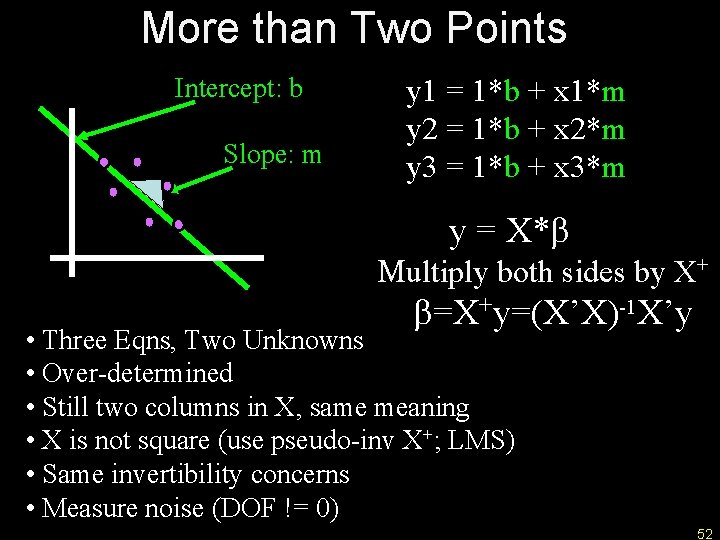
More than Two Points Intercept: b Slope: m y 1 = 1*b + x 1*m y 2 = 1*b + x 2*m y 3 = 1*b + x 3*m y = X*b Multiply both sides by X+ b=X+y=(X’X)-1 X’y • Three Eqns, Two Unknowns • Over-determined • Still two columns in X, same meaning • X is not square (use pseudo-inv X+; LMS) • Same invertibility concerns • Measure noise (DOF != 0) 52

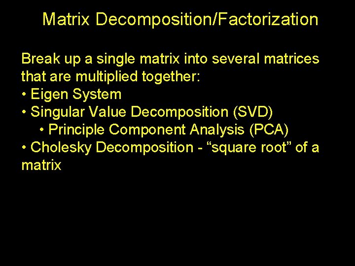
Matrix Decomposition/Factorization Break up a single matrix into several matrices that are multiplied together: • Eigen System • Singular Value Decomposition (SVD) • Principle Component Analysis (PCA) • Cholesky Decomposition - “square root” of a matrix

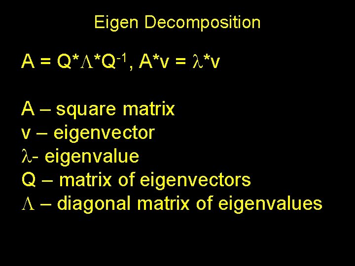
Eigen Decomposition A = Q*L*Q-1, A*v = l*v A – square matrix v – eigenvector l- eigenvalue Q – matrix of eigenvectors L – diagonal matrix of eigenvalues