Matrices Addition of Matrices We add two matrices

Matrices

Addition of Matrices We add two matrices of the same dimensions by adding objects in the same locations in the matrices. For example, • We can think of this as adding respective row vectors, or respective column vectors, of the matrix.

Multiplication by a Scalar • This is the same as multiplying each row vector, or each column vector, by c. As another example,

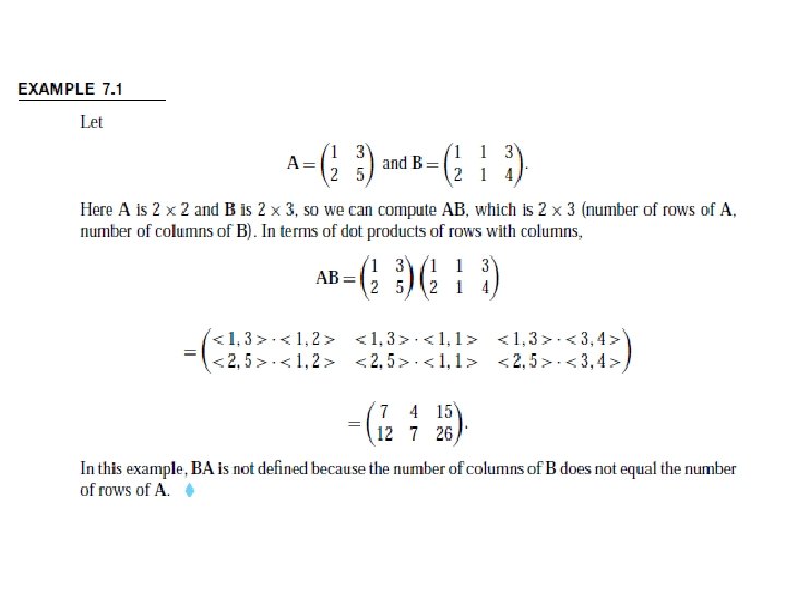
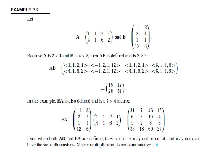
Multiplication of Matrices • This is the dot product of row i of A with column j of B (both are vectors in R ): i, j element of AB=( row i of A) · ( column j of B) • • = (a , · · · , a ) · (b , · · · , b ) • = a b +· · ·+a b. k i 1 i 2 1 j ik i 2 2 j 1 j ik 2 j kj kj • This clarifies why the number of columns of A must equal the number of rows of B for the product AB to be defined. We can only take the dot product of two vectors of the same dimension.

• PROPERTIES: • Let A, B and C be matrices. Then, whenever the indicated operations are defined: • 1. A+B=B+A (matrix addition is commutative). • 2. A(B+C)=AB+AC. • 3. (A+B)C=AC+AC. • 4. (AB)C=A(BC). • 5. c. AB=(c. A)B=A(c. B) for any scalar c.

Terminology and Special Matrices • The n ×m zero matrix O is the n ×m matrix having every element equal to zero. nm • A square matrix is one having the same number of rows and columns. • The n × n identity matrix ; • Thus I has 1 down the main diagonal and zeros everywhere else. n

• Transpose of a Matrix; We form the transpose by interchanging the rows and columns of A. • If A=[a ] is an n ×m matrix, the transpose of A is the m ×n matrix defined by • A =[a ]. ij t ji • Properties of the Transpose

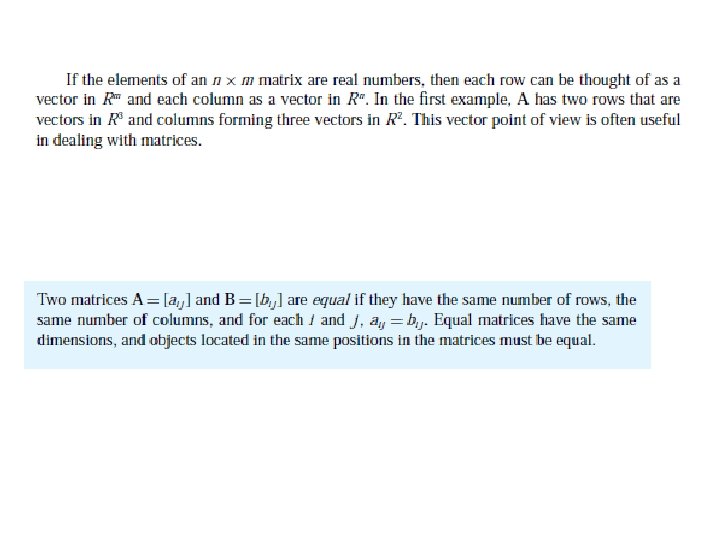
Special Matrices: Symmetric and Skew-Symmetric Matrices • Symmetric matrices are square matrices whose transpose equals the matrix itself. • Skew-symmetric: matrices are square matrices whose transpose equals minus the matrix.

Triangular Matrices. Upper triangular matrices the main diagonal are square matrices that can have nonzero entries only on and above the main diagonal whereas any entry below the diagonal must be zero. Similarly, lower triangular matrices can have nonzero entries only onand below the main diagonal. Any entry on the main diagonal of a triangular matrix may be zero or not.

Diagonal Matrices. These are square matrices that can have nonzero entries only on the main diagonal. Any entry above or below the main diagonal must be zero.

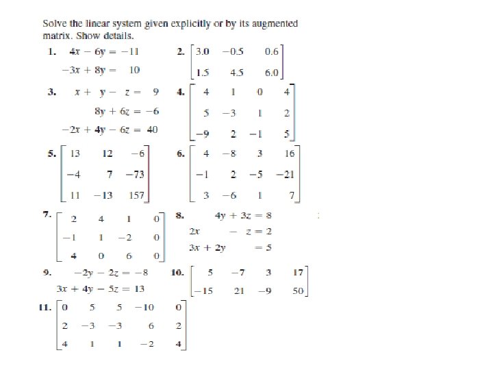
caculate the following expressions or give reasons why they are undefined:

Linear Systems of Equations. Gauss Elimination

• augmented matrix The Gauss elimination method can be motivated as follows. Consider a linear system that is in triangular form (in full, upper triangular form) such as x 2 =26/13 = 2, • This gives us the idea of first reducing a general system to triangular form. For instance, let the given system be

• For this we add twice the first equation to the second, and we do the same operation on the rows of the augmented matrix. This • This is the Gauss elimination (for 2 equations in 2 unknowns) giving the triangular form, from which back substitution now yields x 2 = -2 and x 1 = 6 , as before.

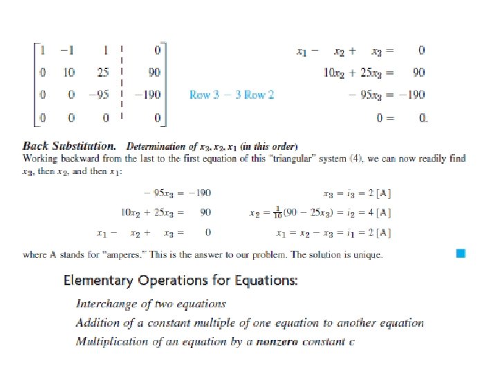
• E X A M P L E : Gauss Elimination: Solve the linear system Step 1. Elimination of x 1 • • • Call the first row of A the pivot row and the first equation the pivot quation Add 1 times the pivot equation to the second equation. Add -20 times the pivot equation to the fourth equation.

• • Add 1 times the pivot equation to the second equation. Add -20 times the pivot equation to the fourth equation • Step 2. Elimination of x 2 Add -3 times the pivot equation to the third equation. The result is

• The Three Possible Cases of Systems

• • E X A M P L E 4 Gauss Elimination if no Solution Exists What will happen if we apply the Gauss elimination to a linear system that has no solution? The answer is that in this case the method will show this fact by producing a contradiction. For instance, consider

• • • (a) No solution. If r is less than m (meaning that R actually has at least one row of all 0 s) and at least one of the numbers fr 1, fr 2, , ﺀ fm is not zero, then the system is inconsistent: No solution is possible (b) Unique solution. If the system is consistent and r=n , there is exactly one solution, which can be found by back substitution. See Example 2, where r=n=3 , m= 4 (c) Infinitely many solutions. To obtain any of these solutions, choose values of arbitrarily. Then solve the rth equation for xr