Introduction to Cosmology Josh Frieman Structure Evolution Cosmology

Introduction to Cosmology Josh Frieman Structure Evolution & Cosmology, Santiago, Oct. 2002

Evolution of the Universe Important to distinguish: 1. What we `know’ (well-established by observations): The Standard Cosmology 2. Speculations/theories that extend beyond the well-established and attempt to explain otherwise unexplained phenomena.

The Big Bang Theory: well-tested framework for understanding the observations and for asking new questions Universe expanding isotropically from a hot, dense `beginning’ (aka the Big Bang) about 14 billion years ago The only successful framework we have for explaining several key facts about the Universe: Hubble’s law of galaxy recession: expansion Uniformity (isotropy) of Microwave background Cosmic abundances of the light elements: Hydrogen, Helium, Deuterium, Lithium, cooked in the first 3 minutes Formation of Large-scale Structure

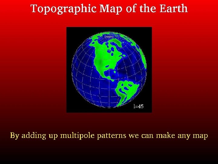
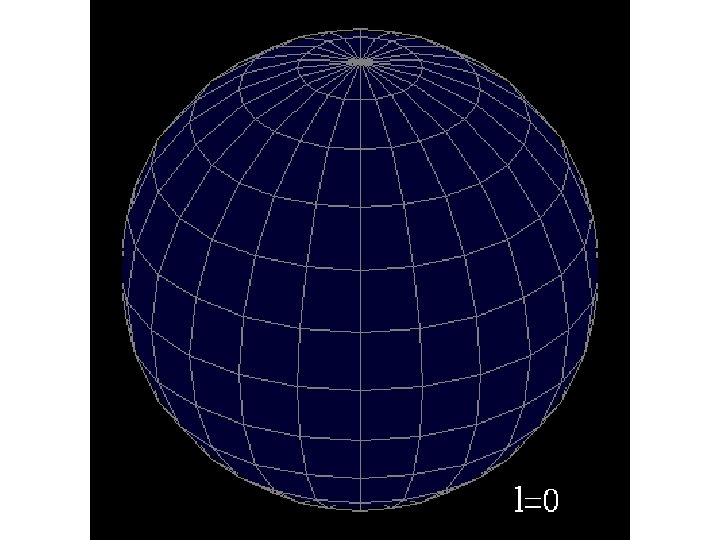
The Big Bang Theory: Status A useful idealization, a simplified description analogous to the approximation of the Earth as a sphere Even so, basic elements of the model remain to be understood: e. g. , the natures of the Dark Matter & Dark Energy which together make up 95% of the mass-energy of the Universe These puzzles do NOT mean that the Big Bang Theory is wrong—rather, it provides the framework for investigating them.

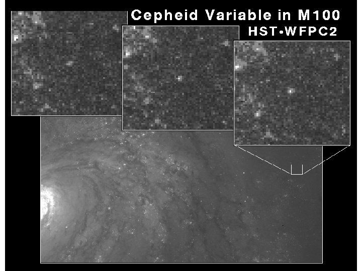
Hubble’s Law and the Expanding Universe Slipher (1922): measured redshifts (recession velocities v) of 40 spiral galaxies by their spectra: Doppler effect Henrietta Leavitt: studied Cepheid variable stars in our Galaxy, showed a correlation between their Luminosity and their Period of variation: L( ) Hubble (1929): found Cepheids in ~20 nearby galaxies and measured their periods inferred L. From their apparent brightness (flux f = L/4πd 2), he obtained their distances d. Comparing the distances d with Slipher’s radial velocities v, he empirically found that v=H 0 d where H 0=550 km/sec/Megaparsec = Hubble’s constant

We observe Hubble law: D v. B=Hd. B v. A=Hd. A By vector addition, v. BA=v. B-v. A =H(d. B-d. A) =Hd. BA B v. BA v. D Us v. A A v. B v 2 v. C Observer A sees Galaxy B C recede according to the Hubble Law as well: Hubble (linear) Law is Universal

`Doppler’ shift of Galaxy Emission/Abs. Lines receding slowly v/c ≈ z = / 0 (approximation for objects moving with v/c << 1) receding quickly

SDSS QSOs

Hubble Space Telescope

Hubble Space Telescope image 40 Cepheids

v = H 0 d + vpec Hubble (1929) Hubble Space Telescope (2000) Freedman, etal

Hubble Diagram extended to larger distances using objects brighter than Cepheids Modern Value: H 0 = 72 8 km/sec/Mpc

Spectrum of the Cosmic Microwave Background Radiation (1965) Photon energy measured by the COBE satellite (1990): no deviations from Blackbody spectrum yet observed

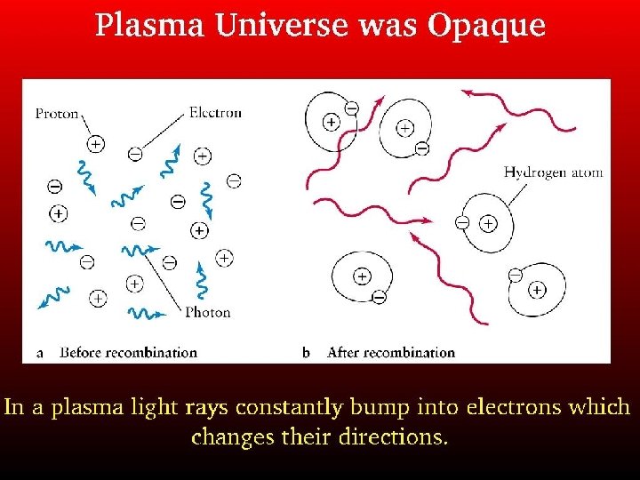
The Microwave Sky: T = 2. 728 K The Universe is filled with relic thermal radiation: Cosmic Microwave Background (CMB) COBE Map of the Temperature of the Universe On large scales, the Universe is (nearly) isotropic around us (the same in all directions): CMB radiation probes as deeply as we can, far beyond optical light from galaxies: snapshot of the young Universe: t = 400, 000 years (z = 1000) recombination Scale of the Observable Universe: Size ~ 1028 cm Mass ~ 1023 Msun

The Microwave Sky: T = 2. 728 K COBE Map of the Temperature of the Universe Dipole anisotropy due to our Galaxy’s peculiar motion through the Universe Red: 2. 7+0. 003 Blue: 2. 7 -0. 003 Red: 2. 7+0. 00001 deg Blue: 2. 7 -0. 00001 deg

The Microwave Sky: T = 2. 728 K COBE Map of the Temperature of the Universe Red: 2. 7+0. 003 Blue: 2. 7 -0. 003 Map with Dipole anisotropy removed: fluctuations of the density of the Universe plus Galactic emission Red: 2. 7+0. 00003 deg Blue: 2. 7 -0. 00003 deg

The Cosmological Principle A working hypothesis (aka the Copernican Principle): We are not priviledged observers at a special place in the Universe: At any instant of time, the Universe should appear ISOTROPIC (over large scales) to All observers. A Universe that appears isotropic to all observers is HOMOGENEOUS i. e. , the same at every location (averaged over large scales).

Statistical homogeneity

Homogeneity & Isotropy: Universe described by single degree of freedom a(t)

2 -D Analogue radius a(t 1): Cosmic Scale Factor radius a(t 2) On average, galaxies are at rest in these expanding (comoving) coordinates

Features of the Expansion of the Universe: • Galaxies and Clusters of galaxies are not expanding with the Universe: they are gravitationally bound systems. • New interpretation of the Redshift of Light: wavelength of light (and all radiation) stretches with expansion: wavelength energy (t) proportional to scale factor a(t) E(t) inversely proportional to a(t) where a(t) is the Cosmic Scale Factor (“radius”) Redshift: 1+z = a(t 0)/a(te) t 0 = age of U today te= age when light was emitted

The Redshift: 1+z = a(t 0)/a(te) = (t 0)/ (te) t 0 = age of U today te = age when light was emitted This expression holds in general, replacing the Doppler formula which held for velocities v << c. No need to talk about recession velocities of galaxies, since they are at rest in the system of expanding coordinates (except for peculiar velocities). (In particular, objects with redshifts z > 1 are not moving faster than the speed of light!)

`Newtonian’ Cosmology How does the `size’ (scale factor) a(t) of the Universe evolve? Consider a homogenous ball of matter (Birkhoff): Kinetic Energy mv 2/2 M d m d a Gravitational Potential Energy -GMm/d (Newton) Conservation of Energy: Kinetic + Potential = Total E = constant mv 2/2 - GMm/d = E density of Universe Now use v=Hd (Hubble) and M= V=(4 /3) d 3 to find H 2 - (8 /3)G = 2 E/md 2 = -k/a 2 Friedmann equation where H= Hubble parameter = expansion rate (H quantifies time rate of change of a(t))

Einstein Cosmology Expansion rate H 2 (da/dt)2/a 2 = (8 /3)G k/a 2 Scale factor Friedmann Spatial curvature Define the critical density: crit = 3 H 02/8 G 1. 9 h 2 x 10 -29 grams/cm 3 and the density parameter: 0 = / crit m ~ a-3 1 - 0 = -k/a 02 H 02 0 > 1 implies k>0 positive spatial curvature 0 = 1 implies k=0 flat 0 < 1 implies k<0 neg. curvature rad ~ a-4

Einstein: space can be globally curved k = +1 k = -1 k=0 What is the geometry of three-dimensional space?

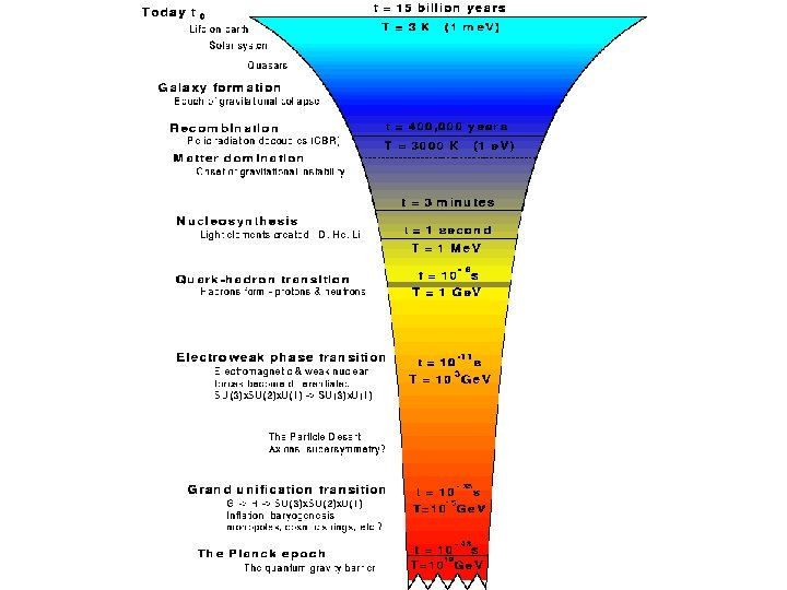
Physical Implications of Expanding Universe An expanding gas cools (TCMB ~ 1/a(t)) and becomes less dense (n ~ 1/a 3(t)) as it expands. Run the expansion backward: going back into the past, the Universe heats up and becomes denser. Expanding Universe plus known laws of physics imply the Universe has finite age and a nearly `singular’ (infinite density and Temperature) beginning about 14 Billion years ago: THE BIG BANG

The Hot Big Bang: relics from the Early Universe How do we test the idea that the early Universe was very hot? Look for relics of this hot phase, observable signatures that require high Temperature (and density) to produce. Best-established signatures: --Cosmic Microwave Background Radiation (CMB) --Abundances of the Light Elements Additional signatures of the Early Universe: --Dark matter particles --Primordial density perturbations which produced CMB anisotropies and (later) galaxies & Large-scale structure --The baryon asymmetry --Topological defects

Dark matter freeze-out Relics produced when their interactions drop out of Thermodynamic Equilibrium: int/H < 1 See talk by Binetruy

Big Bang Nucleosynthesis Origin of the Light Elements: Helium, Deuterium, Lithium, … When t < 1 minute, T > 109 K, atomic nuclei could not survive: the baryons formed a soup of protons & neutrons. As the Temperature dropped below this value (set by the binding energy of light nuclei), protons and neutrons began to fuse together to form bound nuclei: the light elements were synthesized as the Universe expanded and cooled. t(sec) = (k. T/Me. V) 2 during radiation era

Light Element Abundances: predictions Early Universe: protons, neutrons, electrons, neutrinos, photons. Stage 1: t < 1 sec, k. T > 1 Me. V: Weak interactions interconvert neutrons & protons: n p+e+ In equilibrium, n/p = exp( (mn-mp)c 2/k. T). At t ~ 1 sec, weak interactions freeze out ( wk/H < 1), leaving (n/p)F = 1/6. Later, this ratio falls much more slowly due to neutron decay.

Abundance predictions Stage 2: t ~ 1 minute, T ~ 100 ke. V Neutrons and protons fuse to Deuterium (1 neutron+1 proton), Tritium (1 p, 2 n), Helium 4 (2 n, 2 p), and Lithium 7 (3 p, 4 n). Heavier nuclei not produced due to absence of stable mass 5 and 8 elements. By this time, due to neutron decay, n/p ~ 1/7. He 4 is the most stable (most strongly bound) light nucleus, so essentially all the available neutrons end up in He 4 mass fraction Y ~ 2 n/(n+p) ~ 0. 25 25% of the baryonic mass is in Helium, essentially all the rest in Hydrogen, and trace amounts in Deuterium and Lithium.

BBN predicted abundances Fraction of baryonic mass in He 4 Deuterium to Hydrogen ratio h = H 0/(100 km/sec/Mpc) Light Element abundances depend mainly on the density of baryons in the Universe Lithium to Hydrogen ratio baryon/photon ratio

BBN Theory vs. Observations: Observational constraints shown as boxes Remarkable agreement over 10 orders of magnitude in abundance variation Concordance region: b h 2 = 0. 02 0. 001 For h=0. 7, this implies b = 0. 04. Strongest constraint comes from Deuterium (QSO absorption lines) b 4 He

BBN & the Baryon Density Light element abundances are concordant if the baryon (neutron+proton) to photon ratio is about = nb/nphoton = 6 x 10 -10 or bh 2 = 0. 02 (We can make the conversion from to b h 2 since we know the present density of CMB photons, nphoton = 420 per cm 3, very precisely from the CMB Temperature. ) This determination is in excellent agreement with the amplitude of the `acoustic peaks’ in the CMB temperature anisotropy announced last year.

Structure as a Cosmological Probe Paradigm for Structure Formation (SF): Nearly scale-invariant primordial, adiabatic perturbations from inflation, amplified by gravity, in a Universe with (nearly) cold dark matter. While understanding galaxy formation in detail remains difficult (see talk by Silk), the SF paradigm appears robust: confirmed by Large-scale Structure (LSS) and CMB observations. As a result, CMB and LSS now providing sensitive new probes of cosmological parameters.

Recent CMB experiments: Going to smaller angular scales higher resolution

Boomerang Recent CMB Anisotropy Experiments: South Pole DASI

CMB Angular Power Spectrum Statistical way to characterize the spatial structure in a 2 -dimensional image or map T/T = alm Ylm( , ) Cl = <|alm|2> Power spectrum contains all the information if the image is Gaussian

Physics of CMB Anisotropy Acoustic oscillations of the Photon-baryon fluid when the Universe was 400, 000 yrs old Imprint on the Microwave sky Hu

Theoretical dependence of CMB anisotropy on the baryon density Angular frequency Angular separation on the sky

Microwave Background Anisotropy Probes b (Baryon Density) bh 2 = 0. 022 0. 002 Boomerang experiment (2001) DASI experiment (2001)

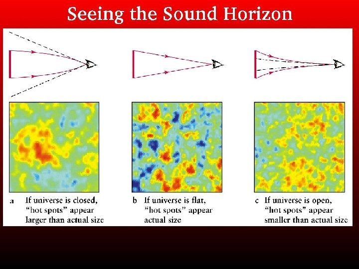
Microwave photons traverse a significant fraction of the Universe, so they can probe its spatial curvature Sizes of hot and cold spots in the CMB give information on curvature of space: In curved space, light bends as it travels: fixed object has larger angular size in a positively curved space: CMB spots appear larger. Opposite occurs for negatively curved space.

Position of first Peak probes the spatial Curvature of the Universe

Microwave Background Anisotropy Probes Spatial Curvature W 0 = 1. 03 0. 06 Boomerang experiment (2001) W 0 = 1. 04 0. 06 DASI experiment (2001)

What is the geometry of space? Recent observations of the Microwave background anisotropy indicate it is nearly flat

Evidence for Dark Matter: Galaxy rotation curves Observed: flat, M ~ d Keplerian: v ~ d-1/2 blueshift redshift Dark halo Typical rotation speed ~200 km/sec and visible disk size ~ 10 kpc Mass ~ 1011 Msun

Clusters of Galaxies: Size ~ 1025 cm ~ Megaparsec (Mpc) Mass ~ 1015 Msun Largest gravitationally bound objects: galaxies, gas, dark matter

Probes of the Matter Density: m (See talks by Reisenegger, Birkinshaw) Current evidence: Galaxy kinematics m ~ 0. 3 Cluster baryons • fb ~ 10 -20% • b h 2 = 0. 02 (BBN/CMB) • m ~ 0. 3 -0. 4 X-ray gas Lensing

m from recent CMB experiments: height of first peak m h 2 = 0. 16 ± 0. 04 (marginalizing over other parameters) Also: m from Large-scale structure and weak lensing (this afternoon) Bridle & Lewis

The 2 Dark Matter Problems Observations indicate: visible matter ~ 0. 01 baryons ~ 0. 04 dark matter ~ 0. 3 BBN+CMB Dark Baryonic matter Dominant component of Dark Matter is Non-baryonic requires a new component beyond quarks, . . .

Basic Dark Matter Questions How much is there? What is the value of m? Current evidence suggests ~ 0. 3. Where is it? Is it just clustered with the luminous material? Not precisely, since Dark halos extend beyond luminous galaxies. Are there completely dark galaxies or clusters? (Some weak lensing studies suggest existence of `dark clumps’. See talk by Miralles) What is it? Evidence from Big Bang Nucleosynthesis suggests most of the DM is not made of baryons. Theory suggests it is a Weakly Interacting Massive elementary Particle (WIMP).

Recent results from Direct WIMP Searches CDMS II now being installed in Soudan gain factor 100 in sensitivity Gaitskell preliminary SUSY

Does Cold Dark Matter predict too much substructure and cuspiness in Galaxy Halos? Dwarf Satellites of the Local Group See talks by Navarro, Teyssier Moore

Halo Substructure and Indirect WIMP Detection Neutralino Annihilation in halo subclumps signal in EGRET, GLAST, VERITAS, … + synchroton signal in CMB Blasi, Olinto, Aloisio (also Bergstrom, etal, Calcaneo-Roldan & Moore, Gondolo & Silk, …)

Halo Substructure and Direct Cold Dark Matter Detection Simulated CDM Clumps & Tidal Streams are coherent in Velocity space Signature of Local Clump/Stream in WIMP Recoil Energy Spectrum Stiff, Widrow, JF

End of Lecture I

Introduction to Cosmology II: Acceleration Past & Present Josh Frieman Structure Evolution & Cosmology, Santiago, Oct. 2002

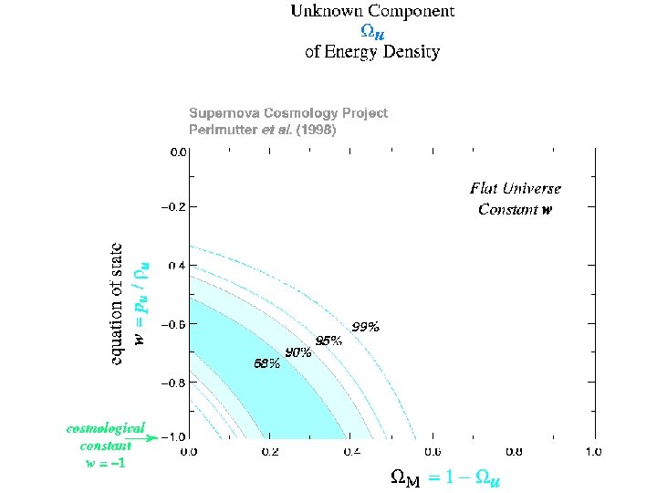
Dark Energy and the Accelerating Universe (c. 1998) Brightness of distant Type Ia supernovae indicates the expansion of the Universe is accelerating, not decelerating. If General Relativity is valid, this requires a new form of stuff with negative effective pressure*: DARK ENERGY Characterize by its equation of state: *more specifically, p < (w < 1/3) pressure w = p/ density

Einstein Cosmology II H 2 = (8 G/3) k/a 2 (1/a 2)(d 2 a/dt 2) = (4 G/3)( +3 p) d /dt + 3(p + )H = 0 Dark Energy: p < 0 d 2 a/dt 2 > 0 Density parameter: 0 = / crit = m + DE ~ a 3(1+w) slower than a-2 0 > 1 (k>0) positive curvature, Univ. recollapses or expands forever 0 = 1 (k=0) flat, expands forever or recollapses 0 < 1 (k<0) negative curvature, expands forever or recollapses

p = (w = 1) Accelerating Size of the Universe What are the densities of Dark matter & Dark Energy? Empty Open Closed Today Cosmic Time

p = (w = 1) Accelerating Size of the Universe SNe Ia + CMB indicate m 0. 3 DE 0. 7 Empty Open Closed Today Cosmic Time

Dark Energy & The Cosmological Constant : a special (and historically first) case of Dark Energy, with p = = constant (w = 1) as the Energy density of the vacuum (empty space): spacetime can be curved even if no matter/radiation particles (or singularities) are present. Einstein: R – (1/2)g R – g = 8 G T (matter) Zel’dovich: R – (1/2)g R = 8 G (T (matter) + T (vac)) vac = / 8 G pvac = – vac = /3 H 02 vac ~ 0. 7 vac ~ (0. 001 e. V)4 [g = (+ – – –)] like a `medium’ with const. energy density and negative pressure

The Cosmological Constant Problem the biggest embarassment for particle physics Classically, can set at will. Quantum zero-point fluctuations: space is not empty, but is filled with virtual particles which continuously fluctuate into and out of the vacuum (via the Uncertainty principle). Vacuum energy density in Quantum Field Theory: vac = /8 G = +/ (1/V) h /2 ~ Include all modes vac = infinity Insert cutoff at kmax = M vac ~ M 4 M hc(k 2+m 2)1/2 d 3 k Pauli

Candidates for the cutoff mass M: MPlanck = 1019 Ge. V scale where classical GR breaks down vac ~ MPlanck 4 ~ 10112 e. V 4 Supersymmetry: boson + fermion contributions to vac cancel, but SUSY must be broken (B and F masses not degenerate) MSUSY ~ 1 Te. V vac ~ 1048 e. V 4 Compare these with the observational constraint on Vacuum energy density: vac < crit ~ 10 -10 e. V 4 Why is the vacuum energy 60 - 120 orders of magnitude smaller than expected? No known symmetry ensures this.

Tragic (Pre-)History of Dark Energy: a cautionary tale Cosmological constant has been periodically invoked to solve cosmological crises, then dropped when they passed: 1916: Einstein: static Universe (`greatest blunder of my life’) 1929: 1 st `age crisis’: Universe (t ~1/H) younger than Earth 1967: apparent clustering of QSOs at fixed redshift 1974: luminosity distance using galaxy std. candles acceleration 1995: 2 nd ‘age crisis’: H 0 = 80 km/sec/Mpc; U. younger than globular clusters 1998: luminosity distance using Sne Ia std. candles acceleration 2000: Spatial flatness from CMB anisotropy Missing energy

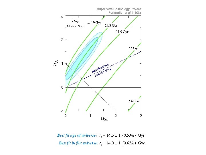
Current Evidence for Dark Energy I. III. IV. Direct Evidence for Acceleration Brightness of distant Type Ia supernovae: Standard candles measure luminosity distance d. L(z sensitive to the expansion history H(z) Supernova Cosmology Project High-Z Supernova Team II. Evidence for `Missing Energy’ CMB Flat Universe: 0 = 1 Clusters, LSS, CMB Low matter density m 0. 3 missing = 1 – 0. 3 = 0. 7 and missing stuff can only dominate recently for structure to form: w < – 0. 5

Discovery of SNe Ia at `high’ redshift z ~ 0. 5 – 1

Intrinsic Brightness vs. Time Physical model: White dwarf star, accreting mass from a companion star, explodes when it exceeds a critical mass (Chandrasekhar) Luminosity Type Ia Supernovae Peak Brightness as a calibrated `Standard’ Candle Time

Type Ia Supernovae Advantages: • small dispersion in peak brightness (std. candles) • single objects (simpler than galaxies) • can be observed over wide z range Challenges: • • • dust (grey dust) causing distant SNe to appear fainter chemical composition evolution of progenitor population photometric calibration environmental differences

Continuing Evidence for Acceleration (m-M) • Riess et al. (2001) SN 1997 ff • NICMOS (HST) serendipitous discovery z = 1. 7

Physical Effects of Dark Energy affects expansion rate of the Universe: Luminosity Distance: d. L(z) = (1+z) dz’/H(z’) Examples: wtot = -1 H = const d ~ z(1+z) (exponential expansion) wtot = 0 H ~ (1+z)3/2 d ~ (1+z)1/2

Apparent Brightness Fainter 42 SNe Ia distance m(z) = M+5 log(H 0 d. L)+K(z)

SNe Ia at z ~ 0. 5 are ~ 0. 2 mag fainter than they would be in an Open Universe with the same value of m

Assuming w= 1 Consistent results from High-Z Team Riess, etal ‘ 98

CMB and Supernovae SNe • de Bernardis et al (2001) • Bridle & Lewis (2002) • orthogonal constraints CMB + H 0 CMB+H+SN +2 d. F+clusters CMB m = 0. 27 = 0. 72 0. 13 0. 11

Concordance Cosmology Our knowledge of the cosmological parameters has made tremendous strides in the last two years: b = 0. 04 (to ~20%) m = 0. 3 (to ~20%) DE = 0. 7 (~15%) total = 1 (~5%) ns = 1 (~10%) H 0 = 72 km/sec/Mpc (~10%) t 0 = 14 Gyr (~8%) baryons matter dark energy slope of power spectrum HST Key Project The prospects for increasing the precision of these measurements in the near future are excellent.

w w DE w w Garnavich etal m

SNe + Clusters ( m > 0. 2) w < 0. 65 (1 )

Combine Constraints Perlmutter, Turner, White ‘ 99 Bean, etal ‘ 01

Age of the Universe H 0 t 0 0. 25 Wm 0. 35 H 0 r/H 0 t 0 • H 0 = 72 • t 0 = 13 8 km/sec/Mpc (Freedman et al. 2001) 1. 5 Gyr (Chaboyer 2001, Krauss 2000) H 0 t 0 = 0. 93 w < -0. 5 0. 15 Huterer & Turner 2001

Dark Energy Models? Cosmological Constant: Vacuum Energy (w = -1) Dynamical scalar fields (w varies) (aka `quintessence’) Frustrated topological defects (w = -1/3 or – 2/3) Replace General Relativity (extra dimensions? )

Two Dark Energy Problems Cosmological constant problem: why is the vacuum energy density 40 -120 orders of magnitude smaller than expected? Coincidence problem: why do we live at the special epoch when the vacuum energy density is comparable to the matter energy density? matter ~ a-3 DE ~ a-3(1+w) matter DE a vac = constant

These two problems are common to ALL Dark Energy models All Dark Energy models assume a (benign) solution of the Cosmological Constant problem

Dynamical Scalar Field Models aka Quintessence General features: meff < 3 H 0 ~ 10 -33 e. V (w < 0) (Potential vs. Kinetic Energy) ~ m 2 2 ~ crit ~ 10 -10 e. V 4 ~ 1028 e. V ~ MPlanck Ultra-light particle: Dark Energy hardly clusters, nearly smooth Equation of state: in general, w > -1 and evolves in time Hierarchy problem: Why m/ ~ 10 -61?

Dynamical Scalar Field Models aka Quintessence Runaway potentials DE/matter constant (Tracker Solution) but coincidence and hierarchy problems remain Pseudo-Nambu Goldstone Boson: Low mass protected by symmetry (ala axion) Frieman, etal V( ) = M 4[1+cos( /f)] f ~ Mplanck M ~ 0. 001 e. V

Key Issues for the Decade 1. Is there Dark Energy? 2. Will the SNe results hold up? 2. What is the nature of the Dark Energy? 3. Is it or something else? 3. How does w = p. X/ X evolve? 4. Dark Energy dynamics Theory

Dark Energy Constraints from on-going Ground-based SN Surveys Huterer CFHTLS, ESSENCE, SDSS, etc

Proposed satellite mission to observe several thousand SNe Ia out to z ~ 1. 7

Determine w to ~ 5%

SNAP SNe Constraints on Dark Energy Evolution JF, Huterer, Linder, Turner

Physical Observables Comoving Distance: r(z) = dx/H(x) In a flat Universe: Luminosity Distance: d. L(z) = r(z)(1+z) Angular diameter Distance: d. A(z) = r(z)/(1+z) Comoving Volume Element: d. V/dzd = r 2(z)/H(z) Linear Perturbation Growth Function: (z)

Complementary Probes of Dark Energy 1. Luminosity distance vs. redshift: d. L(z) Standard candles: SNe Ia m(z) Hubble diagram 2. Angular diameter distance vs. z: d. A(z) Alcock-Paczynski test: Ly-alpha forest; redshift correlations 3. Number counts vs. redshift: N(M, z) probes: *Comoving Volume element d. V/dzd *Growth rate of density perturbations (z) Counts of galaxy halos and of clusters; QSO lensing

Weak Lensing: Cosmic Shear See talk by Refregier Huterer

halos Clusters, shear

The Early Universe: the key to Large-scale Structure From our vantage point 14 billion years after the Big Bang, we are trying to unravel what happened in the earliest tiny fraction of a second, when the Universe was 0. 0000000000000000001 seconds old! We can test our ideas about the Very Early Universe by observing the distributions of galaxies and of cosmic radiations. This has been a major breakthrough in cosmology over the last decade.

Horizons & the CMB COBE showed that the Cosmic Microwave Background is isotropic to 1 part in 105 over the whole sky. Puzzle: regions of the CMB sky separated by more than 1 degree were, at the time of recombination, not yet in causal contact. No reason these causally disconnected regions should have been at the same Temperature! No physical process acting since the Big Bang could have established this uniformity if it wasn’t there at the beginning. Why then does the Universe appear isotropic & homogeneous on large scales? HORIZON PROBLEM

CMB Sky: Points A and B separated by more than few degrees were not in causal contact at decoupling Big Bang t=0 Horizon of observer B at time of decoupling A B 45 o Us, today Photon Decoupling (Last Scattering Surface) t = 400, 000 yr

Structure/Causality Problem Another symptom of the Horizon problem: The Large-scale structures we see today were, at early times, larger than the horizon. The seeds for structure (density perturbations later amplified by gravity) could not have been made causally until very late times (and we have no theory of how to form seeds at late times).

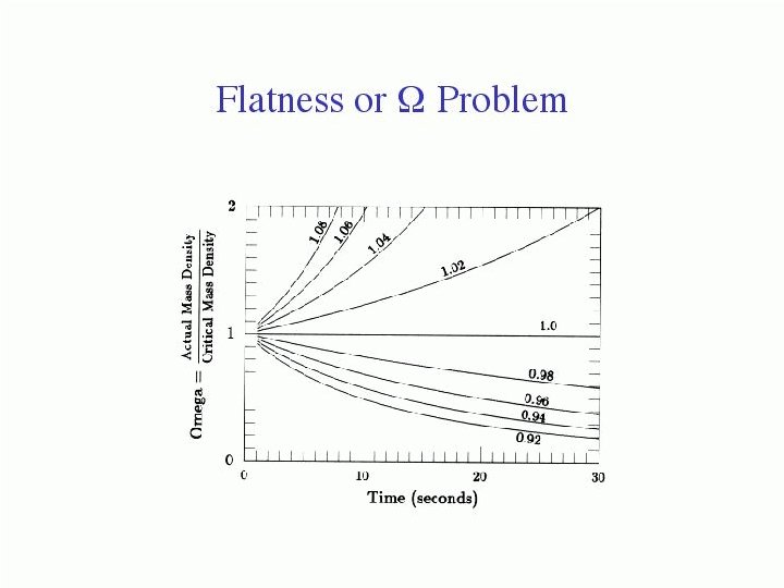
Flatness Problem CMB observations indicate that the observable Universe (within our present horizon) is nearly flat: = 1 As the Universe evolves, the spatial (3 D) curvature generally becomes more important with time: Saddle universe (k = -1) rapidly becomes `empty’; Spherical universe (k = +1) should recollapse rapidly. Natural timescale for these `rapid’ events is the Planck time, t. Planck= LPlanck/c ~ 10 -43 seconds! But our Universe still appears almost flat 1017 sec ~ 1060 Planck times after the Big Bang. Universe must have been `fine tuned’ to be very precisely flat at the Planck time for it still to be roughly flat today.

Problems of Initial Conditions Neither flatness nor homogeneity are `robust’ features of the standard cosmological model: they are unstable conditions. If the early Universe had been slightly more curved or inhomogeneous, it would look much different today. The present state of the observable Universe appears to depend sensitively on the initial state. If we consider an `ensemble’ of Universes at the Planck time, only a tiny fraction of them would evolve to a state that looks like our Universe today. Our observed Universe is in some (hard to quantify) sense very improbable.

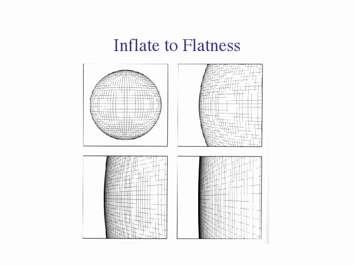
The Inflationary Scenario Theory arose ~1980 (Alan Guth) from thinking about the cosmological consequences of slow symmetry-breaking Phase Transitions in the early Universe. Under certain conditions, a scalar field can get `stuck’ far from its vacuum (ground) state and, if it evolves slowly enough, it can drive an early epoch of very rapid, accelerated expansion. If this accelerated epoch lasts long enough (> 60 e-folds of expansion), it `solves’ the flatness and horizon problems.

Each point in the green dart board represents the initial condition for a possible Universe `God’ may not play dice, but perhaps S/He throws darts. . . Us, now today time Big Bang: t = t. Planck Most Universes look less & less like ours does as they age; God must have been extremely lucky or able to have made our Universe.

During inflation, Homogeneity & Flatness become `attractors’ of the evolution time Us, now Today After inflation Inflation Big Bang Inflation increases the set of initial Universes that end up looking like our Universe today: God could have been lousy at darts.

Inflation Models: Scalar Field slowly rolls down a hill Potential energy density High Temperature: Symmetry is restored, = 0. Low Temperature: Symmetry is broken = + or - field Potential energy function must be fairly `flat’ so the field rolls slowly

After rolling down, scalar field oscillates around the bottom REHEATING Potential energy density High Temperature: Symmetry is restored, = 0. High Temp. Low Temperature: Symmetry is broken = + or - At the end of inflation, the Universe is very cold. field Reheating: Oscillating field energy transformed to other particles as it decays: Universe heats back up to high Temperature: `another’ bang that creates all the matter and energy in the Universe.

Who is the `inflaton’ field? Originally it was thought a GUT Higgs field would do the trick. With the death of old inflation, this hope dimmed. Inflation requires a new scalar field with a very flat potential energy function. Currently, there is no consensus among particle physics theorists as to the identity of this hypothesized inflaton field. Inflation has thus been described as a theory in search of a model.

Density Perturbations & Structure Inflation provides a physical mechanism for producing the initial `seed’ perturbations which grew into Large-scale Structure Density Perturbations from Quantum Mechanics: Classically, scalar field evolves homogeneously: = (t). Quantum Mechanically, the field fluctuates: = (x, t). These field fluctuations imply spatial fluctuations in the energy density of the Universe. During, reheating, these become fluctuations in the density of all matter & radiation particles. The predicted spectrum of density fluctuations now seen to be in excellent agreement with CMB observations: P ~ kn, n 1.

field space field

Scale Quantum density fluctuations are stretched (outside the Hubble radius) to astronomical scales by rapid expansion 3000 Mpc Hubble radius: 1/H(t) 1 Mpc Density Perturbation Length scale of a Galaxy outside inside Before inflation During inflation After inflation Today Time

Power spectrum from inflation During inflation, the only energy scale is H constant. As each scale crosses outside Hubble radius, field perturbations are frozen in, with amplitude |k=H = H/2 Metric perturbations 2 = G ( )2 k = k 3| k|2 H 4 k– 1| k|2 ~ kn– 1 n 1 Density power spectrum

Rolling Inflaton Field Perturbation amplitudes from Inflation Galaxy scale Cluster scale scalar tensor Observable Universe scale

Evidence for Inflation • Large-scale homogeneity and isotropy (by design) • Spatial flatness (Euclidean): total = 1 • (Power) Spectrum of density perturbations inferred from CMB experiments agrees to high precision with spectrum predicted by inflation (n 1) Future: -more precise measurements by satellites (MAP, Planck) -measurement of CMB polarization test inflationary prediction for gravity wave spectrum and distinguish between different inflation models

Microwave Anisotropy Probe (MAP) Satellite Launched by NASA 2001, First results expected December 2002 Finer angular resolution & more sensitive instruments than COBE

CMB Sky: 1992 circa Jan. 2003

MAP Satellite launched June 2001 Planck Satellite planned for ~2008

CMB polarization DASI, 2002: first detection of polarization (E modes) Long term: detection of `B modes’ gravity waves from inflation (challenge: B modes also induced by weak lensing of CMB) See talk by Cooray

First Detection of CMB Polarisation by DASI Results consistent with Anisotropy measurements Kovacs, etal

MAP predicted 1 - errors

Relative Amplitude Of tensor Perturbations

Some Key Questions for 21 st Century Cosmology How did the hierarchy of large-scale structure, from stars to galaxies to clusters and beyond, originate? Did this structure arise from Inflation? What is the nature of the Dark Matter that makes up most of the mass of the Universe? Is it in the form of exotic elementary particles as yet undiscovered? What is the nature of the Dark Energy that is causing the expansion of the Universe to Accelerate? Will the Universe continue to accelerate forever? What happened `before’ the Big Bang? Is this question meaningful? Are there more than 3 spatial dimensions? Can we ever detect them?