Recent developments in nonlinear dimensionality reduction Josh Tenenbaum

Recent developments in nonlinear dimensionality reduction Josh Tenenbaum MIT

Collaborators • • • Vin de Silva John Langford Mira Bernstein Mark Steyvers Eric Berger

Outline • The problem of nonlinear dimensionality reduction • The Isomap algorithm • Development #1: Curved manifolds • Development #2: Sparse approximations

Learning an appearance map • Given input: • Desired output: – Intrinsic dimensionality: 3 – Low-dimensional representation: . . .

Linear dimensionality reduction: PCA, MDS • PCA dimensionality of faces: • First two PCs:

• Linear manifold: PCA • Nonlinear manifold: ?

Previous approaches to nonlinear dimensionality reduction • Local methods seek a set of low-dimensional models, each valid over a limited range of data: – Local PCA – Mixture of factor analyzers • Global methods seek a single low-dimensional model valid over the whole data set: – – – Autoencoder neural networks Self-organizing map Elastic net Principal curves & surfaces Generative topographic mapping

A generative model • • Latent space Y _ Rd Latent data {yi} _ Y generated from p(Y) Mapping f: Yd RN for some N > d Observed data {xi = f (yi)} _ RN Goal: given {xi}, recover f and {yi}.

Chicken-and-egg problem • • We know {xi}. . . and if we knew{yi}, could estimate f. . or if we knew f, could estimate {yi}. So use EM, right? Wrong.

The problem of local minima GTM SOM • Global nonlinear dimensionality reduction + local optimization = severe local minima

A different approach • Attempt to infer {yi} directly from {xi}, without explicit reference to f. • Closed-form, non-iterative, globally optimal solution for {yi}. • Then can approximate f with a suitable interpolation algorithm (RBFs, local linear, . . . ). • In other words, finding f becomes a supervised learning problem on pairs {yi , xi}.

When does this work? • Only given some assumptions on the nature of f and the distribution of the {yi}. • The trick: exploit some invariant of f, a property of the {yi} that is preserved in the {xi}, and that allows the {yi} to be read off uniquely*. * up to some isomorphism (e. g. , rotation).

The assumptions behind three algorithms Distribution: p(Y) Mapping: f Algorithm i) arbitrary linear isometric Classical MDS ii) convex, dense isometric Isomap iii) convex, uniformly dense conformal C-Isomap i) iii) No free lunch: weaker assumptions on f u stronger assumptions on p(Y).

The assumptions behind three algorithms Distribution: p(Y) Mapping: f Algorithm i) arbitrary linear isometric Classical MDS ii) convex, dense isometric Isomap iii) convex, uniformly dense conformal C-Isomap i)

Classical MDS • Invariant: Euclidean distance • Algorithm: – Calculate Euclidean distance matrix D – Convert D to canonical inner product matrix B by “double centering”: – Compute {yi} from eigenvectors of B.

The assumptions behind three algorithms Distribution: p(Y) Mapping: f Algorithm i) arbitrary linear isometric Classical MDS ii) convex, dense isometric Isomap iii) convex, uniformly dense conformal C-Isomap ii)

Isomap • Invariant: geodesic distance

The Isomap algorithm • Construct neighborhood graph G. – e method – K method • Compute shortest paths in G, with edge ij weighted by the Euclidean distance |xi - xj|. – Floyd – Dijkstra (+ Fibonacci heaps) • Reconstruct low-dimensional latent data {yi}. – Classical MDS on graph distances – Sparse MDS with landmarks

Illustration on swiss roll

Discovering the dimensionality • Measure residual variance in geodesic distances. . . MDS / PCA Isomap • . . . and find the elbow.

Theoretical analysis of asymptotic convergence • Conditions for PAC-style asymptotic convergence – Geometric: • Mapping f is isometric to a subset of Euclidean space (i. e. , zero intrinsic curvature). – Statistical: • Latent data {yi} are a “representative” sample* from a convex domain. * Minimum distance from any point on the manifold to a sample point < e (e. g. , variable density Poisson process).

Theoretical results on the rate of convergence • Upper bound on the number of data points required. • Rate of convergence depends on several geometric parameters of the manifold: – Intrinsic: • dimensionality – Embedding-dependent: • minimal radius of curvature • minimal branch separation

Face under varying pose and illumination • Dimensionality • picture MDS / PCA Isomap

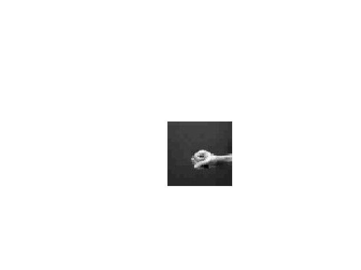
Hand under nonrigid articulation • Dimensionality • picture MDS / PCA Isomap

Apparent motion

Digits • Dimensionality • picture. MDS / PCA Isomap

Summary of Isomap A framework for global nonlinear dimensionality reduction that preserves the crucial features of PCA and classical MDS: • A noniterative, polynomial-time algorithm. • Guaranteed to construct a globally optimal Euclidean embedding. • Guaranteed to converge asymptotically for an important class of nonlinear manifolds. Plus, good results on real and nontrivial synthetic data sets.

Outline • The problem of nonlinear dimensionality reduction • The Isomap algorithm • Development #1: Curved manifolds • Development #2: Sparse approximations

Locally Linear Embedding (LLE) • Roweis and Saul (2000)

Comparing LLE and Isomap • Both start with only local metric information. • Isomap first estimates global metric structure, then finds an embedding that optimally preserves global structure. • LLE finds an embedding that optimally preserves only local structure. • LLE may be more efficient, but may also introduce unpredictable global distortions. • No asymptotic convergence results for LLE.

LLE Isomap

Outline • The problem of nonlinear dimensionality reduction • The Isomap algorithm • Development #1: Curved manifolds • Development #2: Sparse approximations

The assumptions behind three algorithms Distribution: p(Y) Mapping: f Algorithm i) arbitrary linear isometric Classical MDS ii) convex, dense isometric Isomap iii) convex, uniformly dense conformal C-Isomap iii)

Isometric vs. conformal mapping • Isometric map: preserves the Euclidean metric at each point y. • Conformal map: preserves the Euclidean metric at each point y, up to an arbitrary scale factor k(y) > 0. • Properties of conformal maps: – Angle-preserving. – Any subset topologically equivalent to a disk can be conformally mapped onto a disk.

C-Isomap independent of i • Invariant: , , X f Y

The Isomap algorithm • Construct neighborhood graph G. – e method – K method • Compute shortest paths in G, with edge ij weighted by the Euclidean distance |xi - xj|. – Floyd – Dijkstra (+ Fibonacci heaps) • Reconstruct low-dimensional latent data {yi}. – Classical MDS on graph distances – Sparse MDS with landmarks

The C-Isomap algorithm • Construct neighborhood graph G. – e method – K method • Compute shortest paths in G, with edge ij weighted by rescaled distance – Floyd – Dijkstra (+ Fibonacci heaps) • Reconstruct low-dimensional latent data {yi}. – Classical MDS on graph distances – Sparse MDS with landmarks

Conformal fishbowl Data MDS Isomap C-Isomap LLE GTM

Uniform fishbowl Data MDS Isomap C-Isomap LLE GTM

Conformal fishbowl, Gaussian density Latent data C-Isomap LLE

Conformal fishbowl, offset Gaussian density Latent data C-Isomap LLE

Wavelet Data MDS Isomap C-Isomap LLE GTM

Images of Tom’s face . . . • Two intrinsic degrees of freedom: – Translation: left/right – Zoom: in/out • Scale variables (e. g. , zoom) introduce conformal distortion.

Face under translation and zoom Data MDS Isomap C-Isomap LLE GTM

Curvature in LLE vs. Isomap • LLE: +/- Approach: look only at local structure, ignoring global structure. - Asymptotics: unknown. + Nonconformal maps: good for some, but not all. • Isomap: +/- Approach: explicitly estimate, and factor out, local metric distortion (assuming uniform density). + Asymptotics: succeeds for all conformal mappings. + Nonconformal maps: good for some, but not all.