Introduction to Climate forecast System Version 2 CFSV

Introduction to Climate forecast System Version 2 (CFSV 2) – AM, OM, LM, Sea-ice – GODAS and GLDAS Shrinivas Moorthi Acknowledgement; Many of the slides presented here are prepared by members of GCWMB branch and climate and land modeling teams. 12/17/2021 Shrinivas Moorthi 1

Overview • CFS-v 1 description and status • CFS-v 2 CFS Reanalysis and Reforecast (CFSRR) – Atmosphere – Ocean – Land – Sea ice • Future development (CFS-v 3) – Coupled A-O-L-S system – Long term Reanalysis strategy 12/17/2021 Shrinivas Moorthi 2

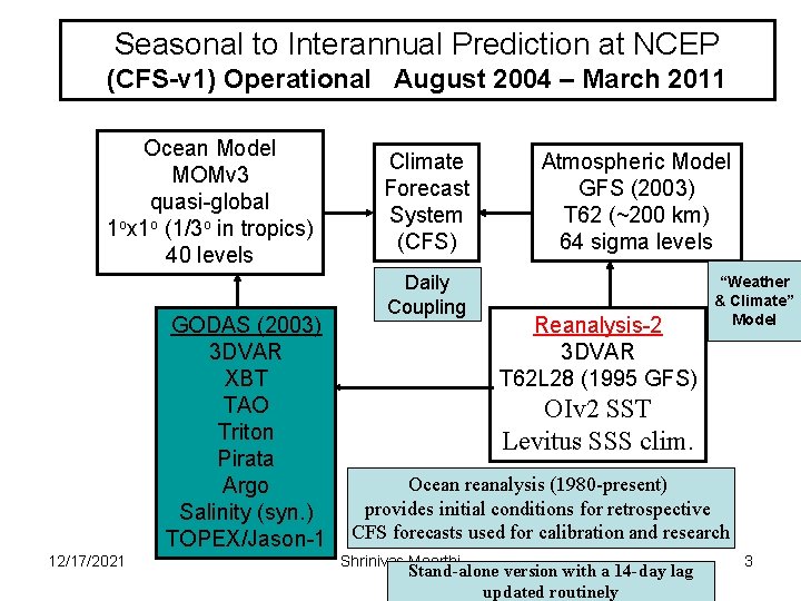
Seasonal to Interannual Prediction at NCEP (CFS-v 1) Operational August 2004 – March 2011 Ocean Model MOMv 3 quasi-global 1 ox 1 o (1/3 o in tropics) 40 levels GODAS (2003) 3 DVAR XBT TAO Triton Pirata Argo Salinity (syn. ) TOPEX/Jason-1 12/17/2021 Climate Forecast System (CFS) Daily Coupling Atmospheric Model GFS (2003) T 62 (~200 km) 64 sigma levels Reanalysis-2 3 DVAR T 62 L 28 (1995 GFS) “Weather & Climate” Model OIv 2 SST Levitus SSS clim. Ocean reanalysis (1980 -present) provides initial conditions for retrospective CFS forecasts used for calibration and research Shrinivas Moorthi Stand-alone version with a 14 -day lag updated routinely 3

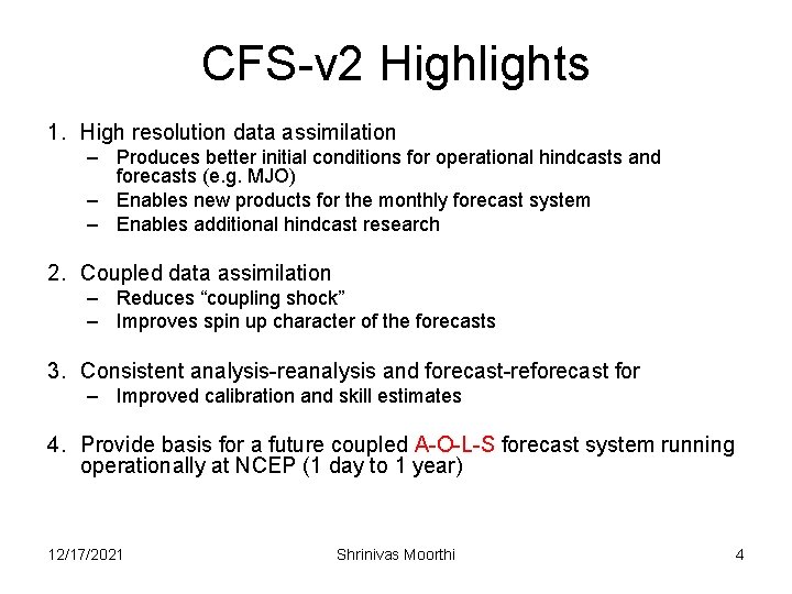
CFS-v 2 Highlights 1. High resolution data assimilation – Produces better initial conditions for operational hindcasts and forecasts (e. g. MJO) – Enables new products for the monthly forecast system – Enables additional hindcast research 2. Coupled data assimilation – Reduces “coupling shock” – Improves spin up character of the forecasts 3. Consistent analysis-reanalysis and forecast-reforecast for – Improved calibration and skill estimates 4. Provide basis for a future coupled A-O-L-S forecast system running operationally at NCEP (1 day to 1 year) 12/17/2021 Shrinivas Moorthi 4

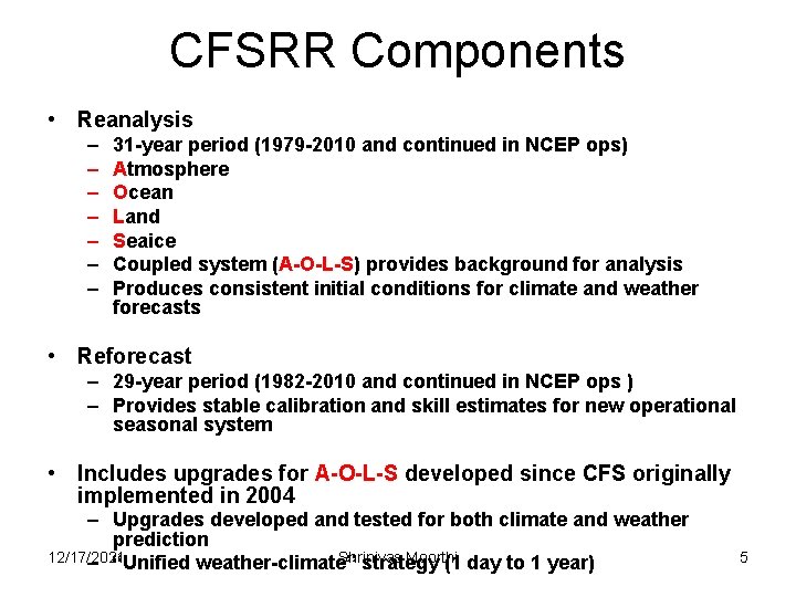
CFSRR Components • Reanalysis – – – – 31 -year period (1979 -2010 and continued in NCEP ops) Atmosphere Ocean Land Seaice Coupled system (A-O-L-S) provides background for analysis Produces consistent initial conditions for climate and weather forecasts • Reforecast – 29 -year period (1982 -2010 and continued in NCEP ops ) – Provides stable calibration and skill estimates for new operational seasonal system • Includes upgrades for A-O-L-S developed since CFS originally implemented in 2004 – Upgrades developed and tested for both climate and weather prediction 12/17/2021 Shrinivas Moorthi – “Unified weather-climate” strategy (1 day to 1 year) 5

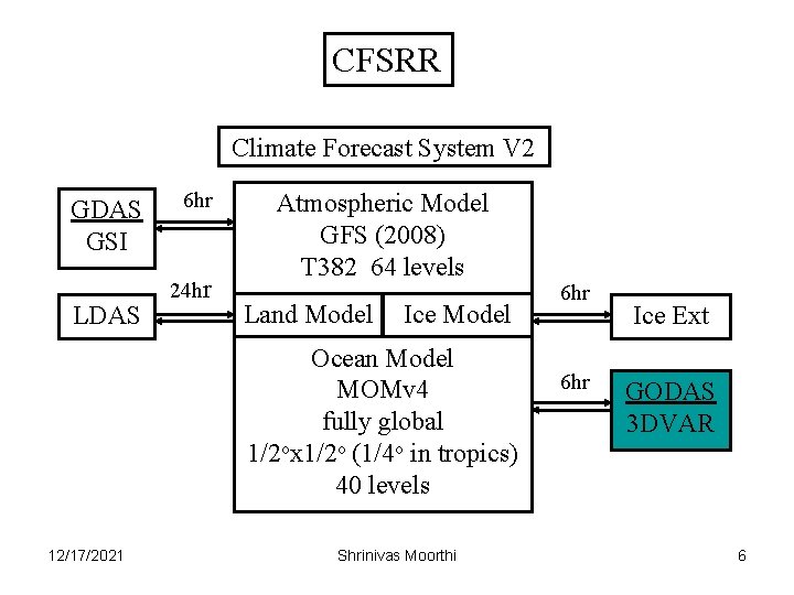
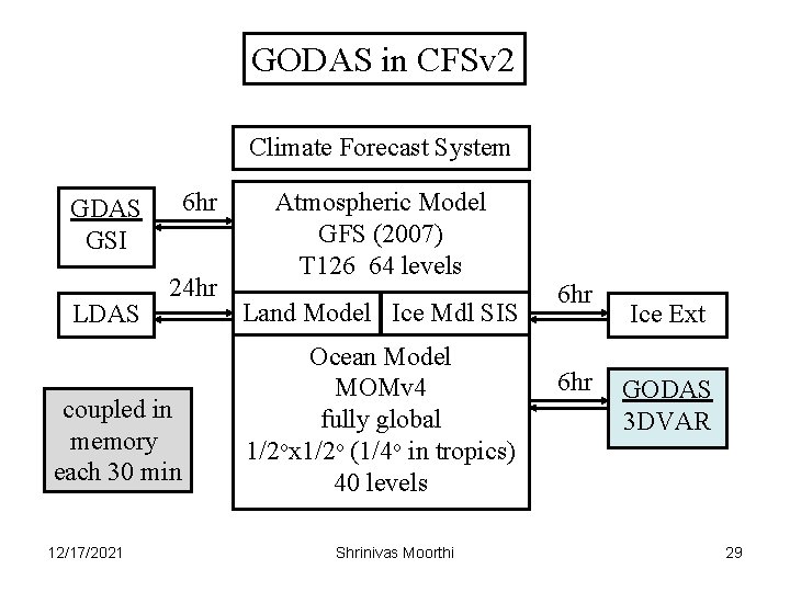
CFSRR Climate Forecast System V 2 GDAS GSI LDAS 6 hr 24 hr Atmospheric Model GFS (2008) T 382 64 levels Land Model Ice Model Ocean Model MOMv 4 fully global 1/2 ox 1/2 o (1/4 o in tropics) 40 levels 12/17/2021 Shrinivas Moorthi 6 hr Ice Ext GODAS 3 DVAR 6

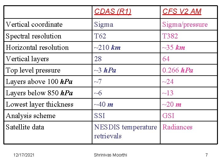
CDAS (R 1) CFS V 2 AM Vertical coordinate Sigma/pressure Spectral resolution T 62 T 382 Horizontal resolution ~210 km ~35 km Vertical layers 28 64 Top level pressure ~3 h. Pa 0. 266 h. Pa Layers above 100 h. Pa ~7 ~24 Layers below 850 h. Pa ~6 ~13 Lowest layer thickness ~40 m ~20 m Analysis scheme SSI GSI Satellite data NESDIS temperature Radiances retrievals 12/17/2021 Shrinivas Moorthi 7

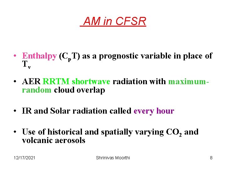
AM in CFSR • Enthalpy (Cp. T) as a prognostic variable in place of Tv • AER RRTM shortwave radiation with maximumrandom cloud overlap • IR and Solar radiation called every hour • Use of historical and spatially varying CO 2 and volcanic aerosols 12/17/2021 Shrinivas Moorthi 8

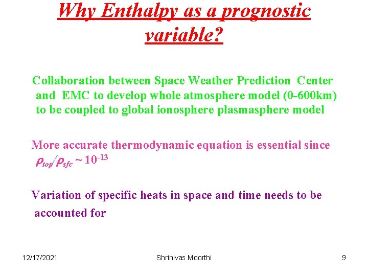
Why Enthalpy as a prognostic variable? Collaboration between Space Weather Prediction Center and EMC to develop whole atmosphere model (0 -600 km) to be coupled to global ionosphere plasmasphere model More accurate thermodynamic equation is essential since rtop/rsfc ~ 10 -13 Variation of specific heats in space and time needs to be accounted for 12/17/2021 Shrinivas Moorthi 9

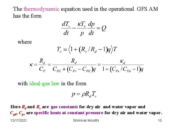
The thermodynamic equation used in the operational GFS AM has the form where with ideal-gas law in the form Here Rd and Rv are gas constants for dry air and water vapor and Cpd, Cpv are specific heats at constant pressure for dry air and water vapor. 12/17/2021 Shrinivas Moorthi 10

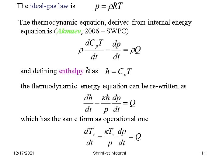
The ideal-gas law is The thermodynamic equation, derived from internal energy equation is (Akmaev, 2006 – SWPC) and defining enthalpy h as thermodynamic energy equation can be re-written as which has the same form as operational one 12/17/2021 Shrinivas Moorthi 11

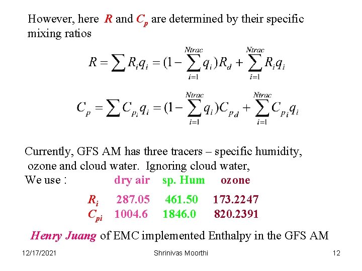
However, here R and Cp are determined by their specific mixing ratios Currently, GFS AM has three tracers – specific humidity, ozone and cloud water. Ignoring cloud water, We use : dry air sp. Hum ozone Ri Cpi 287. 05 1004. 6 461. 50 1846. 0 173. 2247 820. 2391 Henry Juang of EMC implemented Enthalpy in the GFS AM 12/17/2021 Shrinivas Moorthi 12

AM configuration For CDAS • For CDAS vertical coordinate was changed from generalized coordinate of CFSR to sigma-pressure hybrid coordinate of operational GFS. • The vertical advection of tracers based on the TVD scheme is used • Latest version of operational GSI is also used • Convective gravity wave drag and the changes related to marine stratus are retained Other changes made following the current operational GFS are: 12/17/2021 Shrinivas Moorthi 13

AM configuration For CDAS • Resolution and ESMF – Eulerian T 574 L 64 for fcst (0 -9 hr) – ESMF 3. 1. 0 rp 2 • Radiation and cloud – – – – RRTM 2 for Short Wave Radiation RRTM 1 Long Wave Radiation with hourly computation Stratospheric aerosol SW and LW and tropospheric aerosol LW Changing aerosol SW single scattering albedo from 0. 90 in the operation to 0. 99 Changing SW aerosol asymmetry factor. Using new aerosol climatology. Maximum/random cloud overlap Time and spatially varying CO 2 Yang et al. (2008) scheme to treat the dependence of direct-beam surface albedo on solar zenith angle over snow-free land surface 12/17/2021 Shrinivas Moorthi 14

AM Configuration for CDAS • Gravity-Wave Drag Parameterization – Modified GWD routine to automatically scale mountain block and GWD stress with resolution. – Compared to the T 382 L 64 GFS, the T 574 L 64 GFS uses four times stronger mountain block and one half the strength of GWD. • Removal of negative water vapor – Using a positive-definite tracer transport scheme in the vertical to replace the operational central-differencing scheme to eliminate computationally-induced negative tracers. – Changing GSI factqmin and factqmax parameters to reduce negative water vapor and supersaturation points from analysis step. – Modifying cloud physics to limit the borrowing of water vapor that is used to fill negative cloud water to the maximum amount of available water vapor so as to prevent the model from producing negative water vapor. – Changing the minimum value of specific humidity in radiation calculation from 1. 0 e-5 in the operation to 1. 0 e-7 kg/kg. 12/17/2021 Shrinivas Moorthi 15

AM configuration For CDAS • Hurricane relocation – Running hurricane relocation at the 1760 x 880 forecast grid instead of the 1152 x 576 analysis grid – Posting GDAS pgb files first on Guassian grid (1760 x 880), then convert to 0. 5 -deg for hurricane relocation. • Post processing and Utility – Posting GFS forecast master pgb files on 0. 5 deg, then copygb to 1 -deg for postprocessing and archive. – Using a 20 -bit and faster copygb instead of the operational 16 -bit copygb – Using a new chgres which has double precision and has a fix in dry air mass (pdryini 2=0) • Snow analysis Shrinivas Moorthi – Using T 574 compatible high-resolution snow analysis 16 12/17/2021

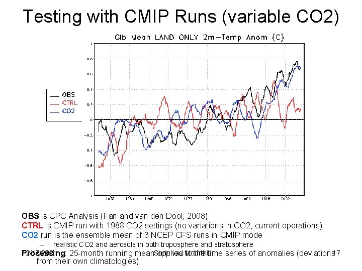
Testing with CMIP Runs (variable CO 2) OBS is CPC Analysis (Fan and van den Dool, 2008) CTRL is CMIP run with 1988 CO 2 settings (no variations in CO 2, current operations) CO 2 run is the ensemble mean of 3 NCEP CFS runs in CMIP mode – realistic CO 2 and aerosols in both troposphere and stratosphere 12/17/2021 Processing: 25 -month running mean. Shrinivas applied Moorthi to the time series of anomalies (deviations 17 from their own climatologies)

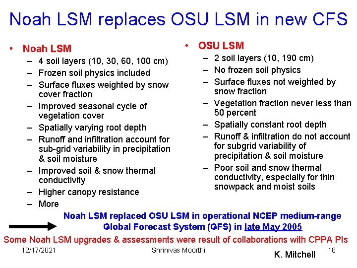
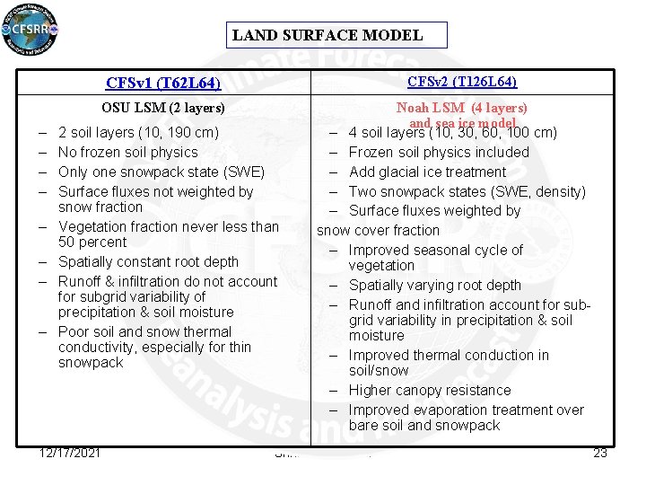
Noah LSM replaces OSU LSM in new CFS • Noah LSM • OSU LSM – 2 soil layers (10, 190 cm) – 4 soil layers (10, 30, 60, 100 cm) – No frozen soil physics – Frozen soil physics included – Surface fluxes not weighted by – Surface fluxes weighted by snow fraction cover fraction – Vegetation fraction never less than – Improved seasonal cycle of 50 percent vegetation cover – Spatially constant root depth – Spatially varying root depth – Runoff & infiltration do not account – Runoff and infiltration account for subgrid variability of sub-grid variability in precipitation & soil moisture – Poor soil and snow thermal – Improved soil & snow thermal conductivity, especially for thin conductivity snowpack and moist soils – Higher canopy resistance – More Noah LSM replaced OSU LSM in operational NCEP medium-range Global Forecast System (GFS) in late May 2005 Some Noah LSM upgrades & assessments were result of collaborations with CPPA PIs 12/17/2021 Shrinivas Moorthi K. Mitchell 18

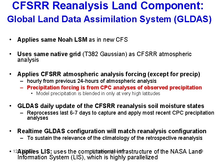
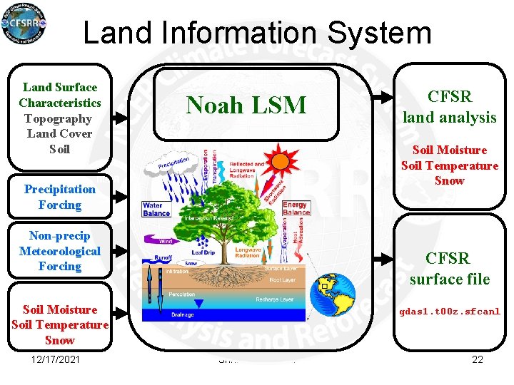
CFSRR Reanalysis Land Component: Global Land Data Assimilation System (GLDAS) • Applies same Noah LSM as in new CFS • Uses same native grid (T 382 Gaussian) as CFSRR atmospheric analysis • Applies CFSRR atmospheric analysis forcing (except for precip) – hourly from previous 24 -hours of atmospheric analysis – Precipitation forcing is from CPC analyses of observed precipitation • Model precipitation is blended in only at very high latitudes • GLDAS daily update of the CFSRR reanalysis soil moisture states – Reprocesses last 6 -7 days to capture and apply most recent CPC precipitation analyses • Realtime GLDAS configuration will match reanalysis configuration – To sustain the relevance of the climatology of the retrospective reanalysis Shrinivas Moorthi 19 • 12/17/2021 Applies LIS: uses the computational infrastructure of the NASA Land Information System (LIS), which is highly parallelized

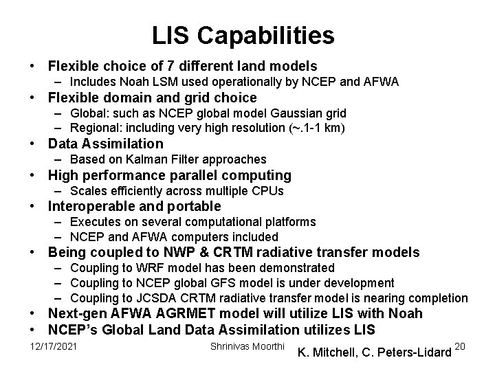
LIS Capabilities • Flexible choice of 7 different land models – Includes Noah LSM used operationally by NCEP and AFWA • Flexible domain and grid choice – Global: such as NCEP global model Gaussian grid – Regional: including very high resolution (~. 1 -1 km) • Data Assimilation – Based on Kalman Filter approaches • High performance parallel computing – Scales efficiently across multiple CPUs • Interoperable and portable – Executes on several computational platforms – NCEP and AFWA computers included • Being coupled to NWP & CRTM radiative transfer models – Coupling to WRF model has been demonstrated – Coupling to NCEP global GFS model is under development – Coupling to JCSDA CRTM radiative transfer model is nearing completion • Next-gen AFWA AGRMET model will utilize LIS with Noah • NCEP’s Global Land Data Assimilation utilizes LIS 12/17/2021 Shrinivas Moorthi K. Mitchell, C. Peters-Lidard 20

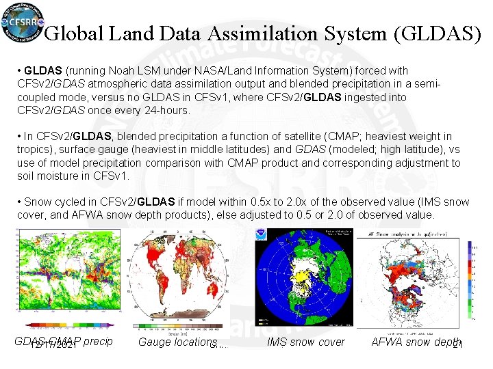
Global Land Data Assimilation System (GLDAS) • GLDAS (running Noah LSM under NASA/Land Information System) forced with CFSv 2/GDAS atmospheric data assimilation output and blended precipitation in a semicoupled mode, versus no GLDAS in CFSv 1, where CFSv 2/GLDAS ingested into CFSv 2/GDAS once every 24 -hours. • In CFSv 2/GLDAS, blended precipitation a function of satellite (CMAP; heaviest weight in tropics), surface gauge (heaviest in middle latitudes) and GDAS (modeled; high latitude), vs use of model precipitation comparison with CMAP product and corresponding adjustment to soil moisture in CFSv 1. • Snow cycled in CFSv 2/GLDAS if model within 0. 5 x to 2. 0 x of the observed value (IMS snow cover, and AFWA snow depth products), else adjusted to 0. 5 or 2. 0 of observed value. GDAS-CMAP 12/17/2021 precip Gauge locations IMS snow cover Shrinivas Moorthi AFWA snow depth 21

Land Information System Land Surface Characteristics Topography Land Cover Soil Noah LSM Soil Moisture Soil Temperature Snow Precipitation Forcing Non-precip Meteorological Forcing CFSR surface file Land Variables Soil Moisture Soil Temperature Snow 12/17/2021 CFSR land analysis gdas 1. t 00 z. sfcanl Shrinivas Moorthi Christa Peters-Lidard et al. , NASA/GSFC/HSB 22

LAND SURFACE MODEL CFSv 2 (T 126 L 64) CFSv 1 (T 62 L 64) OSU LSM (2 layers) – – – – 2 soil layers (10, 190 cm) No frozen soil physics Only one snowpack state (SWE) Surface fluxes not weighted by snow fraction Vegetation fraction never less than 50 percent Spatially constant root depth Runoff & infiltration do not account for subgrid variability of precipitation & soil moisture Poor soil and snow thermal conductivity, especially for thin snowpack 12/17/2021 Noah LSM (4 layers) and sea ice model – 4 soil layers (10, 30, 60, 100 cm) – Frozen soil physics included – Add glacial ice treatment – Two snowpack states (SWE, density) – Surface fluxes weighted by snow cover fraction – Improved seasonal cycle of vegetation – Spatially varying root depth – Runoff and infiltration account for subgrid variability in precipitation & soil moisture – Improved thermal conduction in soil/snow – Higher canopy resistance – Improved evaporation treatment over bare soil and snowpack Shrinivas Moorthi 23

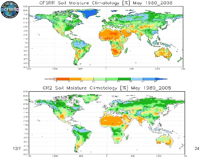
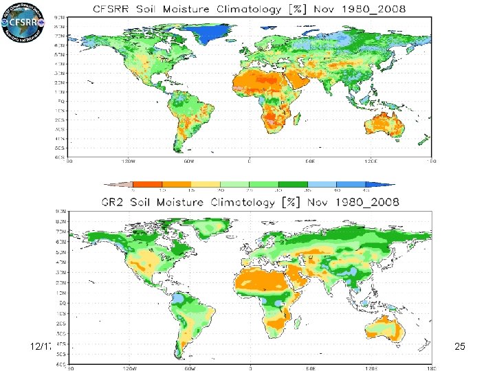
CFSR Soil Moisture Climatology 12/17/2021 Shrinivas Moorthi 24

CFSR Soil Moisture Climatology 12/17/2021 Shrinivas Moorthi 25

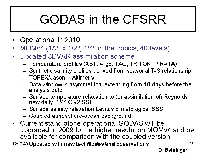
GODAS in the CFSRR • Operational in 2010 • MOMv 4 (1/2 o x 1/2 o, 1/4 o in the tropics, 40 levels) • Updated 3 DVAR assimilation scheme – – Temperature profiles (XBT, Argo, TAO, TRITON, PIRATA) Synthetic salinity profiles derived from seasonal T-S relationship TOPEX/Jason-1 Altimetry Data window is asymmetrical extending from 10 -days before the analysis date – Surface temperature relaxation to (or assimilation of) Reynolds new daily, 1/4 o OIv 2 SST – Surface salinity relaxation Levitus climatological SSS – Coupled atmosphere-ocean background • Current stand-alone operational GODAS will be upgraded in 2009 to the higher resolution MOMv 4 and be available for comparison with the coupled version 12/17/2021 – Updated Shrinivas Moorthi with new techniques and observations 26 D. Behringer

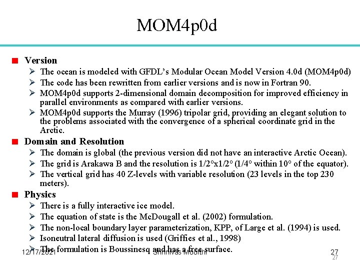
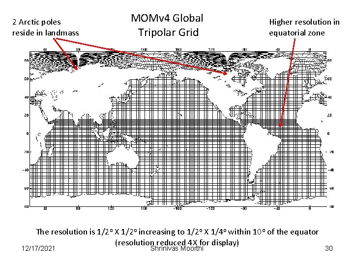
MOM 4 p 0 d Version Ø The ocean is modeled with GFDL’s Modular Ocean Model Version 4. 0 d (MOM 4 p 0 d) Ø The code has been rewritten from earlier versions and is now in Fortran 90. Ø MOM 4 p 0 d supports 2 -dimensional domain decomposition for improved efficiency in parallel environments as compared with earlier versions. Ø MOM 4 p 0 d supports the Murray (1996) tripolar grid, providing an elegant solution to the problems associated with the convergence of a spherical coordinate grid in the Arctic. Domain and Resolution Ø The domain is global (the previous version did not have an interactive Arctic Ocean). Ø The grid is Arakawa B and the resolution is 1/2 ox 1/2 o (1/4 o within 10 o of the equator). Ø The vertical grid has 40 Z-levels with variable resolution (23 levels in the top 230 meters). Physics Ø There is a fully interactive ice model. Ø The equation of state is the Mc. Dougall et al. (2002) formulation. Ø The non-local boundary layer parameterization, KPP, of Large et al. (1994) is used. Ø Isoneutral lateral diffusion is used (Griffies et al. , 1998) Ø The formulation is Boussinesq and has a. Moorthi free surface. 12/17/2021 Shrinivas 27 27

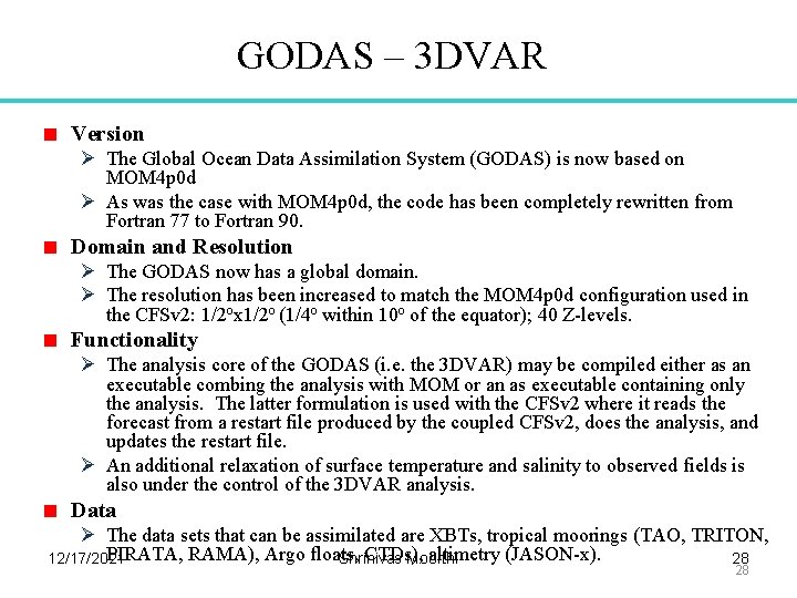
GODAS – 3 DVAR Version Ø The Global Ocean Data Assimilation System (GODAS) is now based on MOM 4 p 0 d Ø As was the case with MOM 4 p 0 d, the code has been completely rewritten from Fortran 77 to Fortran 90. Domain and Resolution Ø The GODAS now has a global domain. Ø The resolution has been increased to match the MOM 4 p 0 d configuration used in the CFSv 2: 1/2 ox 1/2 o (1/4 o within 10 o of the equator); 40 Z-levels. Functionality Ø The analysis core of the GODAS (i. e. the 3 DVAR) may be compiled either as an executable combing the analysis with MOM or an as executable containing only the analysis. The latter formulation is used with the CFSv 2 where it reads the forecast from a restart file produced by the coupled CFSv 2, does the analysis, and updates the restart file. Ø An additional relaxation of surface temperature and salinity to observed fields is also under the control of the 3 DVAR analysis. Data Ø The data sets that can be assimilated are XBTs, tropical moorings (TAO, TRITON, PIRATA, RAMA), Argo floats, CTDs), altimetry (JASON-x). 12/17/2021 Shrinivas Moorthi 28 28

GODAS in CFSv 2 Climate Forecast System GDAS GSI LDAS 6 hr 24 hr coupled in memory each 30 min 12/17/2021 Atmospheric Model GFS (2007) T 126 64 levels Land Model Ice Mdl SIS Ocean Model MOMv 4 fully global 1/2 ox 1/2 o (1/4 o in tropics) 40 levels Shrinivas Moorthi 6 hr Ice Ext GODAS 3 DVAR 29

2 Arctic poles reside in landmass MOMv 4 Global Tripolar Grid Higher resolution in equatorial zone The resolution is 1/2 o X 1/2 o increasing to 1/2 o X 1/4 o within 10 o of the equator (resolution reduced 4 X for display) 12/17/2021 Shrinivas Moorthi 30

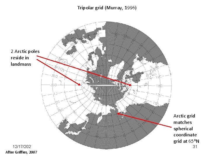
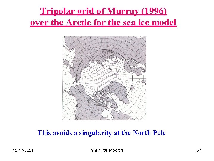
Tripolar grid (Murray, 1996) 2 Arctic poles reside in landmass Arctic grid matches spherical coordinate grid at 65 o. N 12/17/2021 After Griffies, 2007 Shrinivas Moorthi 31

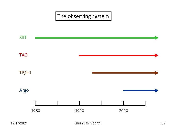
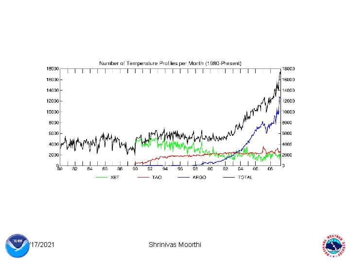
The observing system XBT TAO TP/J-1 Argo 1980 12/17/2021 1990 Shrinivas Moorthi 2000 32

12/17/2021 Shrinivas Moorthi 33

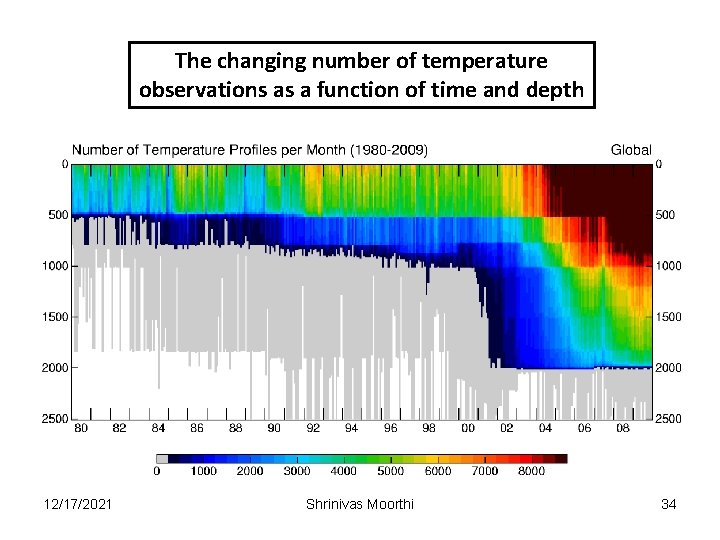
The changing number of temperature observations as a function of time and depth 12/17/2021 Shrinivas Moorthi 34

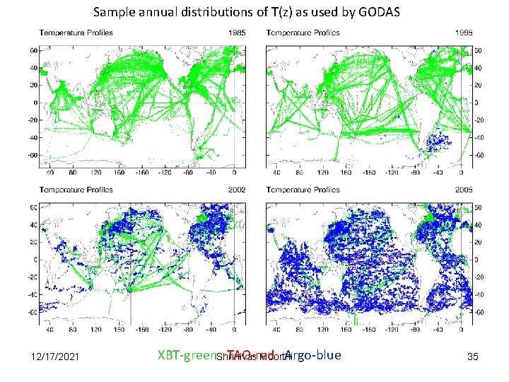
Sample annual distributions of T(z) as used by GODAS 12/17/2021 XBT-green. Shrinivas TAO-red Argo-blue Moorthi 35

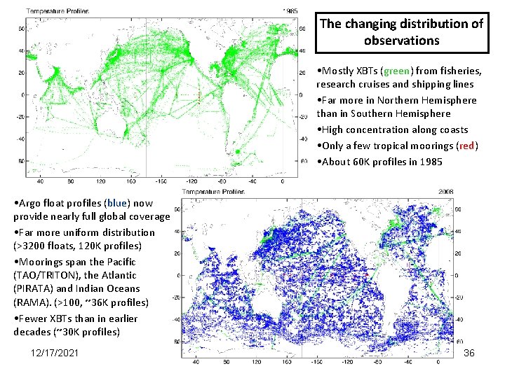
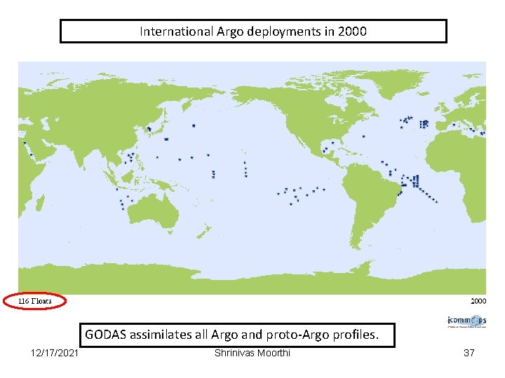
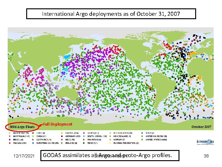
The changing distribution of observations • Mostly XBTs (green) from fisheries, research cruises and shipping lines • Far more in Northern Hemisphere than in Southern Hemisphere • High concentration along coasts • Only a few tropical moorings (red) • About 60 K profiles in 1985 • Argo float profiles (blue) now provide nearly full global coverage • Far more uniform distribution (>3200 floats, 120 K profiles) • Moorings span the Pacific (TAO/TRITON), the Atlantic (PIRATA) and Indian Oceans (RAMA). (>100, ~36 K profiles) • Fewer XBTs than in earlier decades (~30 K profiles) 12/17/2021 Shrinivas Moorthi 36

International Argo deployments in 2000 GODAS assimilates all Argo and proto-Argo profiles. 12/17/2021 Shrinivas Moorthi 37

International Argo deployments as of October 31, 2007 Full Deployment 12/17/2021 GODAS assimilates all. Shrinivas Argo and proto-Argo profiles. Moorthi 38

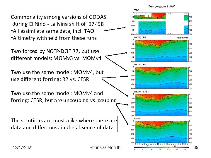
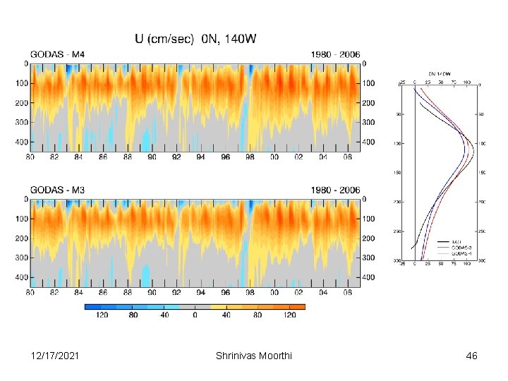
Commonality among versions of GODAS during El Nino - La Nina shift of ‘ 97 -’ 98 • All assimilate same data, incl. TAO • Altimetry withheld from these runs Two forced by NCEP-DOE R 2, but use different models: MOMv 3 vs. MOMv 4 Two use the same model: MOMv 4, but use different forcing: R 2 vs. CFSR Two use the same model: MOMv 4 and forcing: CFSR, but are uncoupled vs. coupled The solutions are most alike where there are data and differ most in the absence of data. 12/17/2021 Shrinivas Moorthi 39

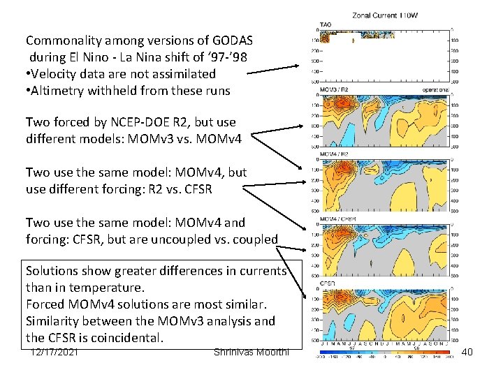
Commonality among versions of GODAS during El Nino - La Nina shift of ‘ 97 -’ 98 • Velocity data are not assimilated • Altimetry withheld from these runs Two forced by NCEP-DOE R 2, but use different models: MOMv 3 vs. MOMv 4 Two use the same model: MOMv 4, but use different forcing: R 2 vs. CFSR Two use the same model: MOMv 4 and forcing: CFSR, but are uncoupled vs. coupled Solutions show greater differences in currents than in temperature. Forced MOMv 4 solutions are most similar. Similarity between the MOMv 3 analysis and the CFSR is coincidental. 12/17/2021 Shrinivas Moorthi 40

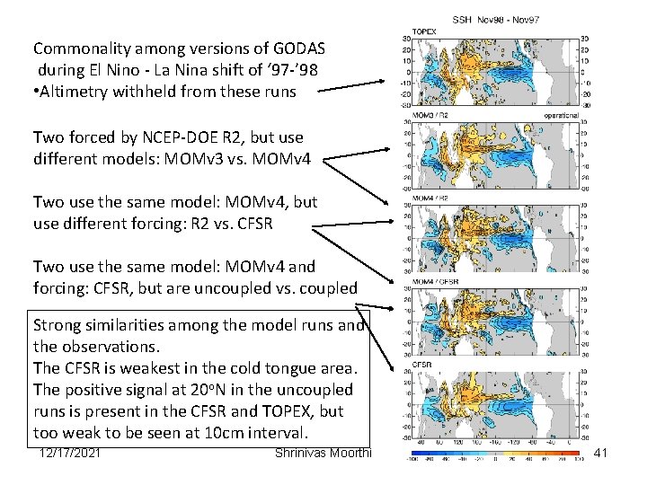
Commonality among versions of GODAS during El Nino - La Nina shift of ‘ 97 -’ 98 • Altimetry withheld from these runs Two forced by NCEP-DOE R 2, but use different models: MOMv 3 vs. MOMv 4 Two use the same model: MOMv 4, but use different forcing: R 2 vs. CFSR Two use the same model: MOMv 4 and forcing: CFSR, but are uncoupled vs. coupled Strong similarities among the model runs and the observations. The CFSR is weakest in the cold tongue area. The positive signal at 20 o. N in the uncoupled runs is present in the CFSR and TOPEX, but too weak to be seen at 10 cm interval. 12/17/2021 Shrinivas Moorthi 41

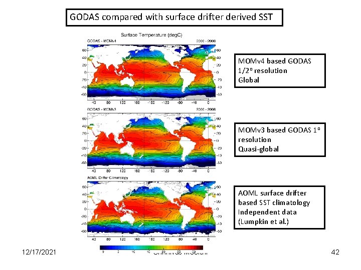
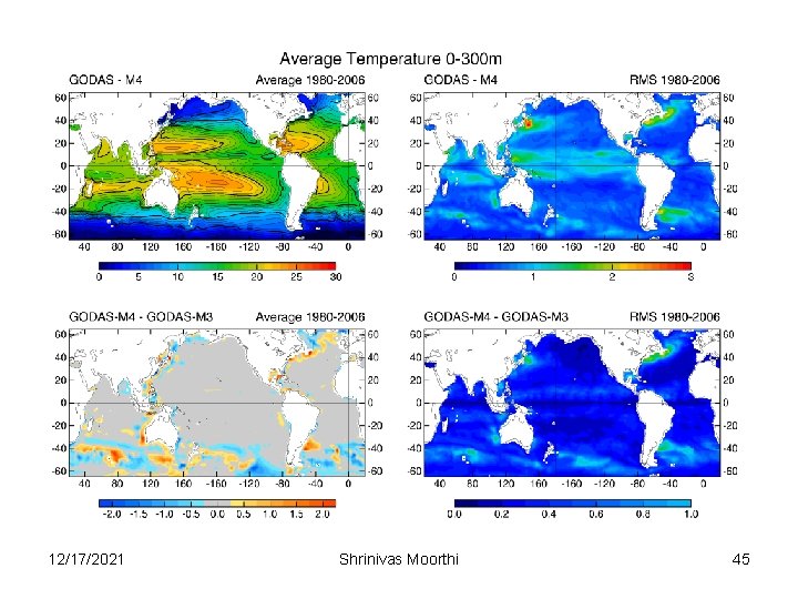
GODAS compared with surface drifter derived SST MOMv 4 based GODAS 1/2 o resolution Global MOMv 3 based GODAS 1 o resolution Quasi-global AOML surface drifter based SST climatology Independent data (Lumpkin et al. ) 12/17/2021 Shrinivas Moorthi 42

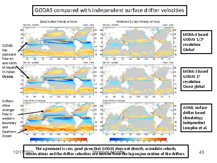
GODAS compared with independent surface drifter velocities GODAS has eastward flow on and north of equator in Indian Ocean Drifters show stronger flow in western boundary and Southern Ocean MOMv 4 based GODAS 1/2 o resolution Global MOMv 3 based GODAS 1 o resolution Quasi-global AOML surface drifter based climatology Independent Lumpkin et al. The agreement is very good given that GODAS does not directly assimilate velocity 12/17/2021 Shrinivas observations and the drifter velocities are derived. Moorthi from the lagrangian motion of the drifters. 43

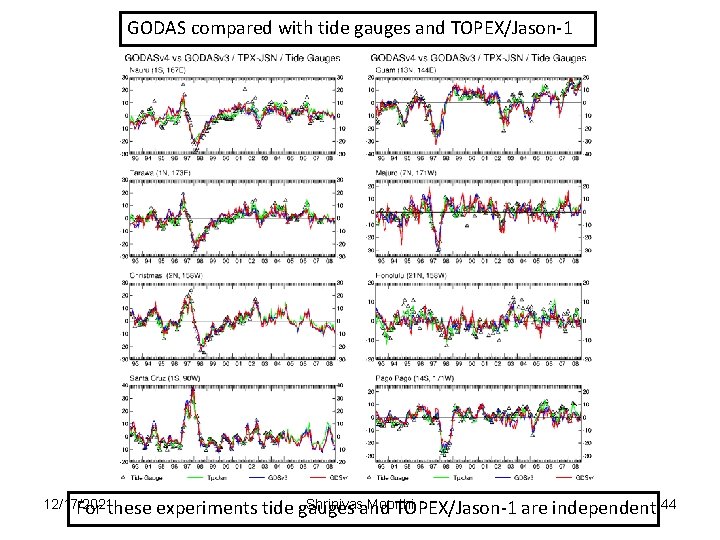
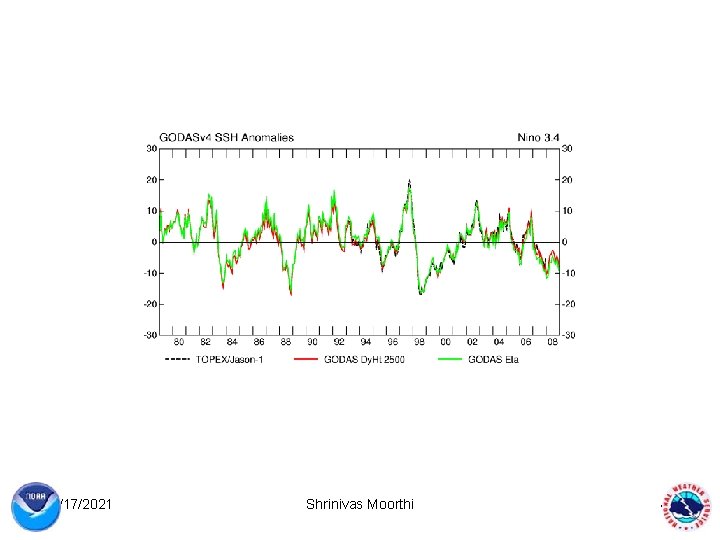
GODAS compared with tide gauges and TOPEX/Jason-1 12/17/2021 For these Shrinivasand Moorthi experiments tide gauges TOPEX/Jason-1 are independent 44

12/17/2021 Shrinivas Moorthi 45

12/17/2021 Shrinivas Moorthi 46

12/17/2021 Shrinivas Moorthi 47

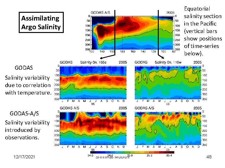
Equatorial salinity section in the Pacific (vertical bars show positions of time-series below). Assimilating Argo Salinity GODAS Salinity variability due to correlation with temperature. GODAS-A/S Salinity variability introduced by observations. 12/17/2021 Shrinivas Moorthi 48

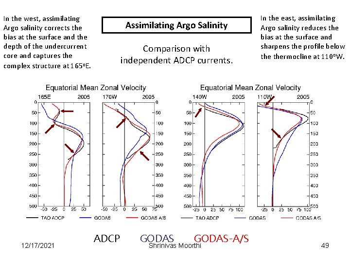
In the west, assimilating Argo salinity corrects the bias at the surface and the depth of the undercurrent core and captures the complex structure at 165 o. E. 12/17/2021 Assimilating Argo Salinity Comparison with independent ADCP currents. ADCP GODAS-A/S Shrinivas Moorthi In the east, assimilating Argo salinity reduces the bias at the surface and sharpens the profile below thermocline at 110 o. W. 49

INCOIS – NCEP Collaboration Co-Principal Investigators: M. Ravichandran (INCOIS), D. Behringer (NCEP) The collaboration was established in November of 2009 for the purpose of transferring a copy of NCEP’s Global Ocean Data Assimilation System (GODAS) to INCOIS. The GODAS will provide INCOIS with a real-time analysis of the physical state of the Indian Ocean through the assimilation of data sets from a variety of platforms (ships, moorings, autonomous drifting buoys, satellite). In return, NCEP will benefit from an ongoing expert evaluation of the GODAS performance in the Indian Ocean, leading to model and system improvements. GODAS code and sample forcing and assimilation data suitable for testing were transferred to INCOIS in January, 2010. INCOIS had GODAS up and running by the end of March and had finished a long experiment (2003 – present) by the end of April. INCOIS is currently exploring the sensitivity of the system to the wind forcing (NCEP vs Quik. SCAT). 12/17/2021 Shrinivas Moorthi 50

SEA ICE Model in CFSV 2 Xingren Wu EMC/NCEP and IMSG 12/17/2021 Shrinivas Moorthi 51

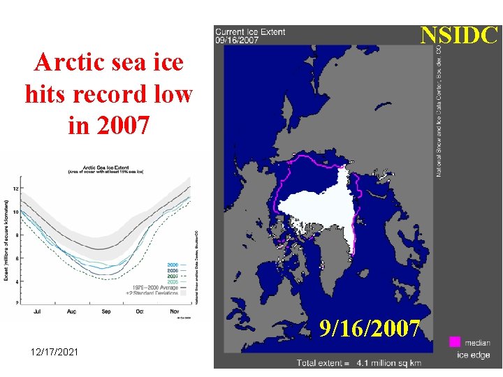
NSIDC Arctic sea ice hits record low in 2007 9/16/2007 12/17/2021 Shrinivas Moorthi 52

Outline • Sea Ice in the Weather and Climate System • Sea Ice in the NCEP Forecast System - Analysis/Assimilation - Forecast: GFS, CFS • Sea Ice in the CFS Reanalysis 12/17/2021 Shrinivas Moorthi 53

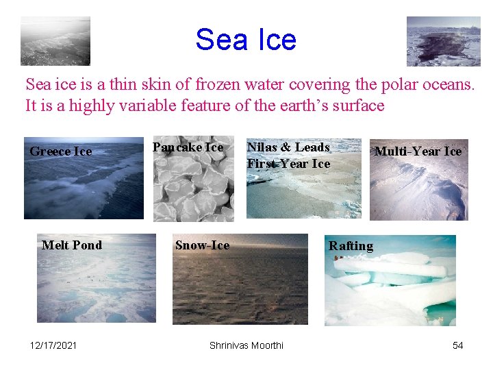
Sea Ice Sea ice is a thin skin of frozen water covering the polar oceans. It is a highly variable feature of the earth’s surface. Greece Ice Melt Pond 12/17/2021 Pancake Ice Nilas & Leads First-Year Ice Snow-Ice Shrinivas Moorthi Multi-Year Ice Rafting 54

Sea ice affects climate and weather related processes Ø Sea ice amplifies any change of climate due to its “positive feedback” (coupled climate model concern): Sea ice is white and reflects solar radiation back to space. More sea ice cools the Earth, less of it warms the Earth. A cooler Earth means more sea ice and vice versa. Ø Sea ice restricts the exchange of heat/water between the air and ocean (NWP concern) ØSea ice modifies air/sea momentum transfer, ocean fresh water balance and ocean circulation: The formation of sea ice injects salt into the ocean which makes the water heavier and causes it to flow downwards to the deep waters and drive a massive ocean circulation 12/17/2021 Shrinivas Moorthi 55

Issues related to sea ice forecast v Data assimilation v Initial conditions v Sea ice models and coupling 12/17/2021 Shrinivas Moorthi 56

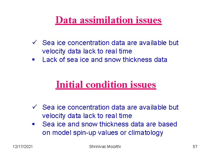
Data assimilation issues ü Sea ice concentration data are available but velocity data lack to real time § Lack of sea ice and snow thickness data Initial condition issues ü Sea ice concentration data are available but velocity data lack to real time § Sea ice and snow thickness data are based on model spin-up values or climatology 12/17/2021 Shrinivas Moorthi 57

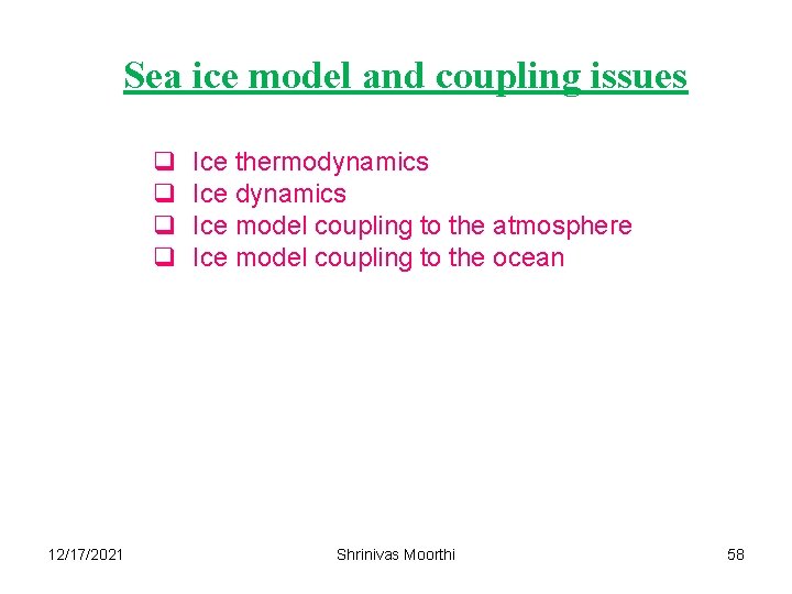
Sea ice model and coupling issues q q 12/17/2021 Ice thermodynamics Ice model coupling to the atmosphere Ice model coupling to the ocean Shrinivas Moorthi 58

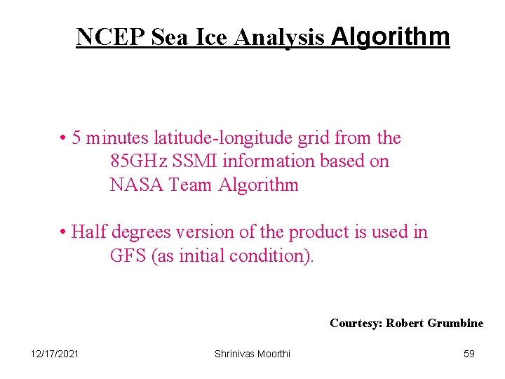
NCEP Sea Ice Analysis Algorithm • 5 minutes latitude-longitude grid from the 85 GHz SSMI information based on NASA Team Algorithm • Half degrees version of the product is used in GFS (as initial condition). Courtesy: Robert Grumbine 12/17/2021 Shrinivas Moorthi 59

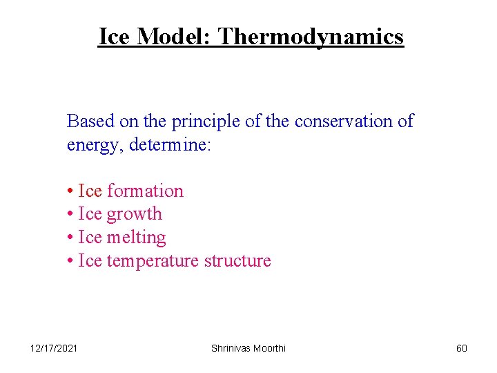
Ice Model: Thermodynamics Based on the principle of the conservation of energy, determine: • Ice formation • Ice growth • Ice melting • Ice temperature structure 12/17/2021 Shrinivas Moorthi 60

Ice Model: Dynamics Based on the principle of the conservation of momentum, determine: • Ice motions • Ice deformation • Leads (open water) 12/17/2021 Shrinivas Moorthi 61

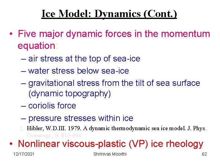
Ice Model: Dynamics (Cont. ) • Five major dynamic forces in the momentum equation: – air stress at the top of sea-ice – water stress below sea-ice – gravitational stress from the tilt of sea surface (dynamic topography) – coriolis force – pressure stresses within ice 1. Hibler, W. D. III. 1979. A dynamic thermodynamic sea ice model. J. Phys. Oceanogr. , 9, 815 -846 • Nonlinear viscous-plastic (VP) ice rheology 12/17/2021 Shrinivas Moorthi 62

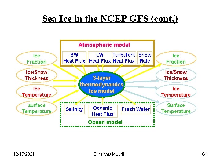
Sea Ice in the NCEP Global Forecast System • A three-layer thermodynamic sea ice model was embedded into GFS (May 2005). • It predicts sea ice/snow thickness, the surface temperature and ice temperature structure. • In each model grid box, the heat and moisture fluxes and albedo are treated separately for ice and open water. 12/17/2021 Shrinivas Moorthi 63

Sea Ice in the NCEP GFS (cont. ) Atmospheric model Ice Fraction Ice/Snow Thickness Ice Temperature surface Temperature SW LW Turbulent Snow Heat Flux Rate 3 -layer thermodynamics Ice model Salinity Oceanic Heat Flux Fresh Water Ice Fraction Ice/Snow Thickness Ice Temperature Surface Temperature Ocean model 12/17/2021 Shrinivas Moorthi 64

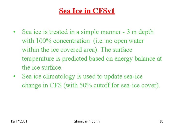
Sea Ice in CFSv 1 • Sea ice is treated in a simple manner - 3 m depth with 100% concentration (i. e. no open water within the ice covered area). The surface temperature is predicted based on energy balance at the ice surface. • Sea ice climatology is used to update sea-ice change in CFS (with 50% cutoff for sea-ice cover). 12/17/2021 Shrinivas Moorthi 65

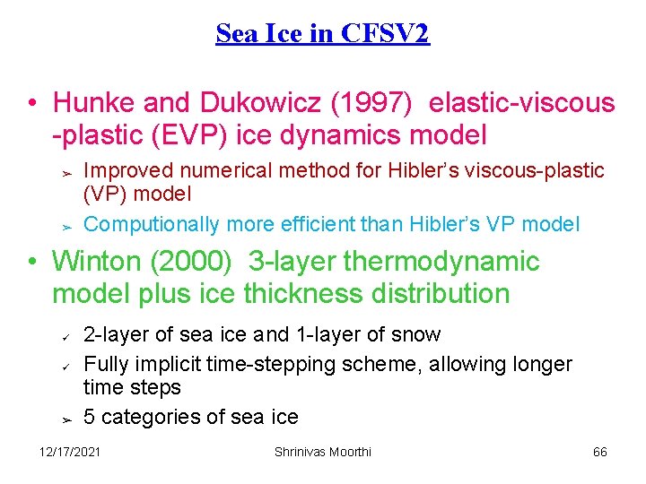
Sea Ice in CFSV 2 • Hunke and Dukowicz (1997) elastic-viscous -plastic (EVP) ice dynamics model ➢ ➢ Improved numerical method for Hibler’s viscous-plastic (VP) model Computionally more efficient than Hibler’s VP model • Winton (2000) 3 -layer thermodynamic model plus ice thickness distribution ü ü ➢ 2 -layer of sea ice and 1 -layer of snow Fully implicit time-stepping scheme, allowing longer time steps 5 categories of sea ice 12/17/2021 Shrinivas Moorthi 66

Tripolar grid of Murray (1996) over the Arctic for the sea ice model This avoids a singularity at the North Pole 12/17/2021 Shrinivas Moorthi 67

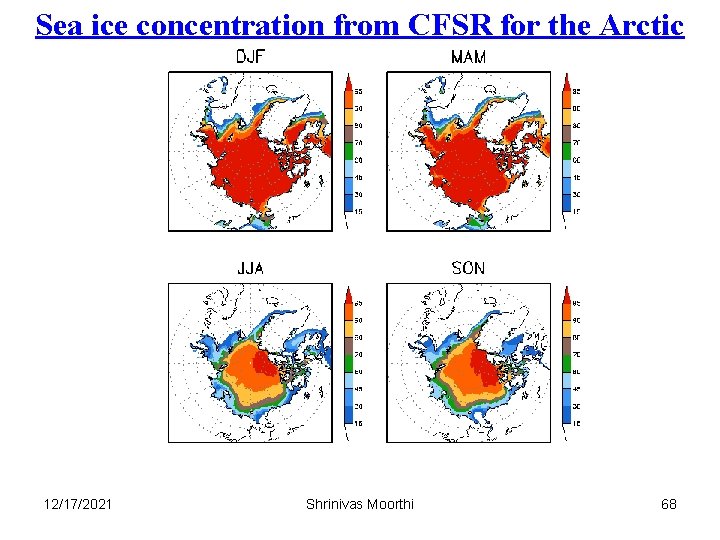
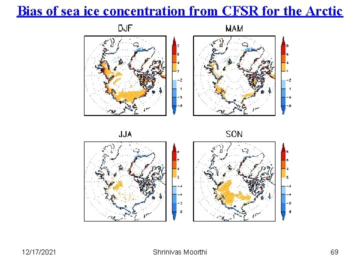
Sea ice concentration from CFSR for the Arctic 12/17/2021 Shrinivas Moorthi 68

Bias of sea ice concentration from CFSR for the Arctic 12/17/2021 Shrinivas Moorthi 69

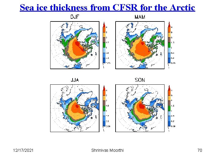
Sea ice thickness from CFSR for the Arctic 12/17/2021 Shrinivas Moorthi 70

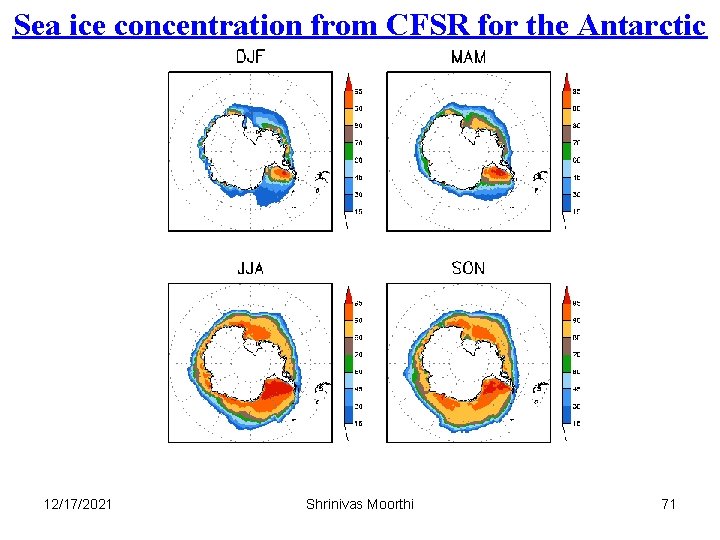
Sea ice concentration from CFSR for the Antarctic 12/17/2021 Shrinivas Moorthi 71

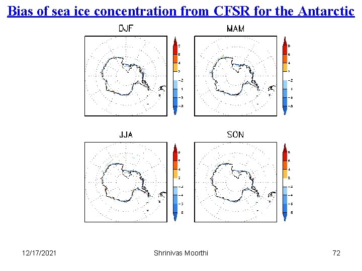
Bias of sea ice concentration from CFSR for the Antarctic 12/17/2021 Shrinivas Moorthi 72

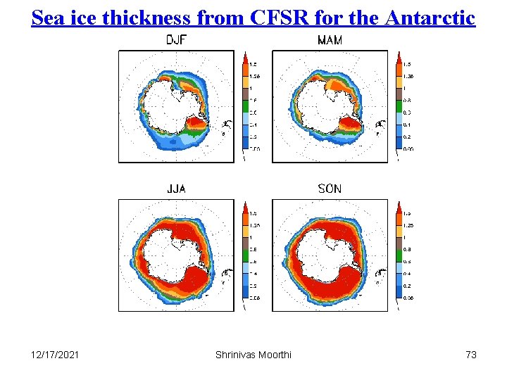
Sea ice thickness from CFSR for the Antarctic 12/17/2021 Shrinivas Moorthi 73

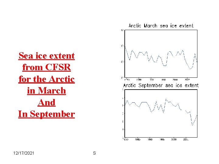
Sea ice extent from CFSR for the Arctic in March And In September 12/17/2021 Shrinivas Moorthi 74

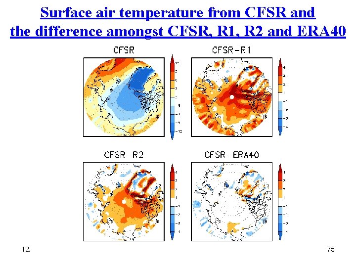
Surface air temperature from CFSR and the difference amongst CFSR, R 1, R 2 and ERA 40 12/17/2021 Shrinivas Moorthi 75

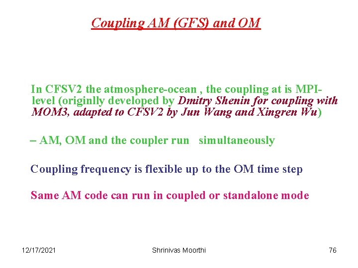
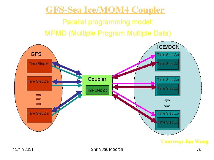
Coupling AM (GFS) and OM In CFSV 2 the atmosphere-ocean , the coupling at is MPIlevel (originlly developed by Dmitry Shenin for coupling with MOM 3, adapted to CFSV 2 by Jun Wang and Xingren Wu) – AM, OM and the coupler run simultaneously Coupling frequency is flexible up to the OM time step Same AM code can run in coupled or standalone mode 12/17/2021 Shrinivas Moorthi 76

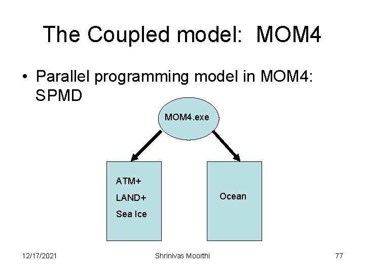
The Coupled model: MOM 4 • Parallel programming model in MOM 4: SPMD MOM 4. exe ATM+ Ocean LAND+ Sea Ice 12/17/2021 Shrinivas Moorthi 77

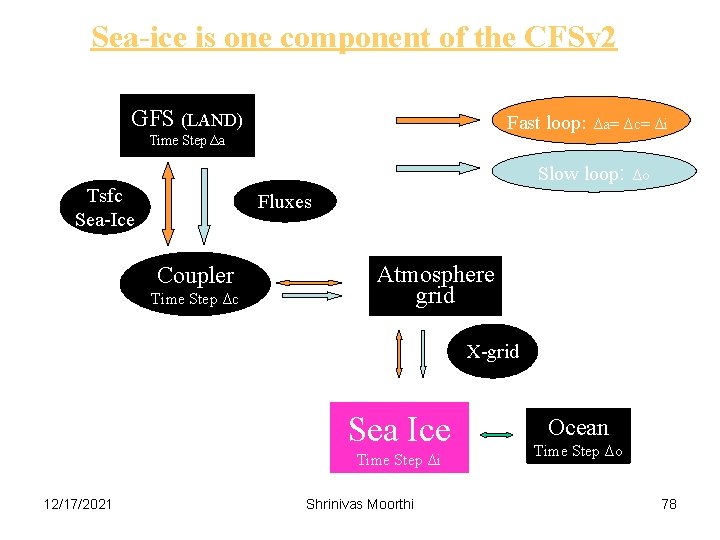
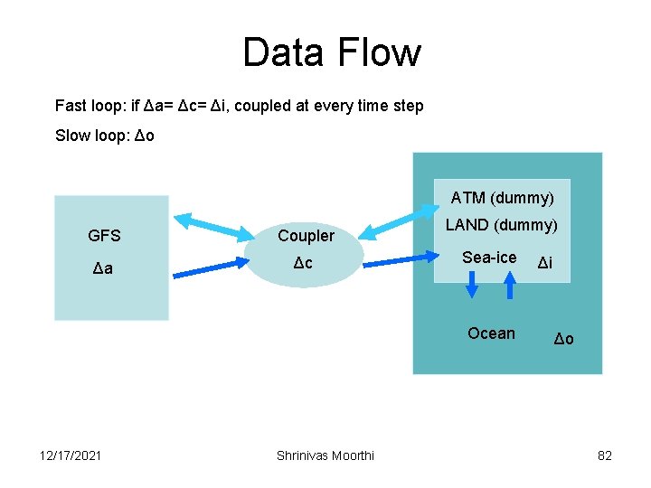
Sea-ice is one component of the CFSv 2 GFS (LAND) Fast loop: Time Step Δa Δa= Δc= Δi Slow loop: Tsfc Sea-Ice Δo Fluxes Coupler Time Step Δc Atmosphere grid X-grid Sea Ice Time Step Δi 12/17/2021 Shrinivas Moorthi Ocean Time Step Δo 78

GFS-Sea Ice/MOM 4 Coupler Parallel programming model: MPMD (Multiple Program Multiple Data) ICE/OCN GFS Time Step Δo Time Step Δa Time Step Δi Coupler Time Step Δo Time Step Δc Time Step Δi Time Step Δa Time Step Δo Time Step Δi Courtesy: Jun Wang 12/17/2021 Shrinivas Moorthi 79

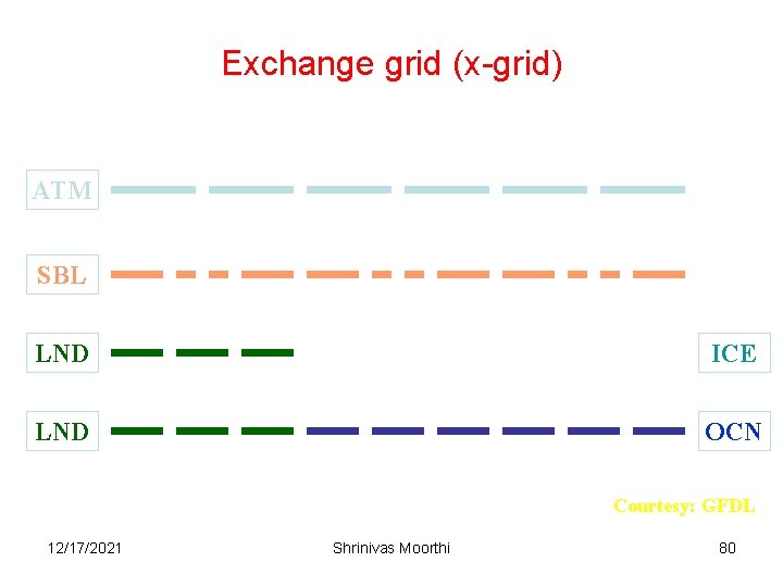
Exchange grid (x-grid) ATM SBL LND ICE LND OCN Courtesy: GFDL 12/17/2021 Shrinivas Moorthi 80

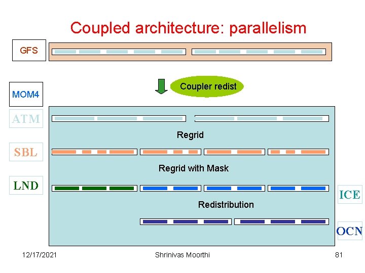
Coupled architecture: parallelism GFS MOM 4 Coupler redist ATM Regrid SBL Regrid with Mask LND Redistribution ICE OCN 12/17/2021 Shrinivas Moorthi 81

Data Flow Fast loop: if Δa= Δc= Δi, coupled at every time step Slow loop: Δo ATM (dummy) GFS Coupler Δa Δc LAND (dummy) Sea-ice Ocean 12/17/2021 Shrinivas Moorthi Δi Δo 82

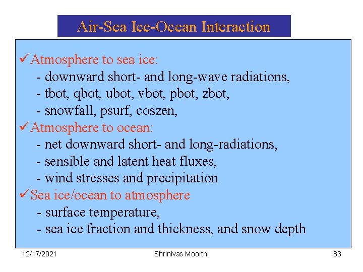
Air-Sea Ice-Ocean Interaction üAtmosphere to sea ice: - downward short- and long-wave radiations, - tbot, qbot, ubot, vbot, pbot, zbot, - snowfall, psurf, coszen, üAtmosphere to ocean: - net downward short- and long-radiations, - sensible and latent heat fluxes, - wind stresses and precipitation üSea ice/ocean to atmosphere - surface temperature, - sea ice fraction and thickness, and snow depth 12/17/2021 Shrinivas Moorthi 83

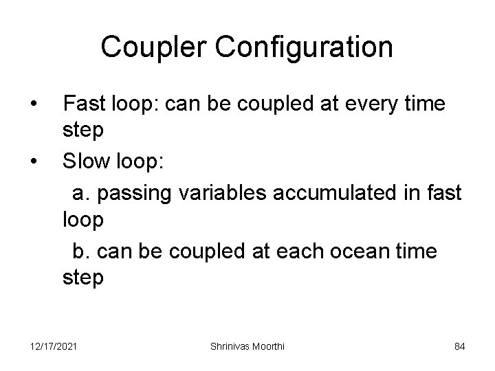
Coupler Configuration • • Fast loop: can be coupled at every time step Slow loop: a. passing variables accumulated in fast loop b. can be coupled at each ocean time step 12/17/2021 Shrinivas Moorthi 84

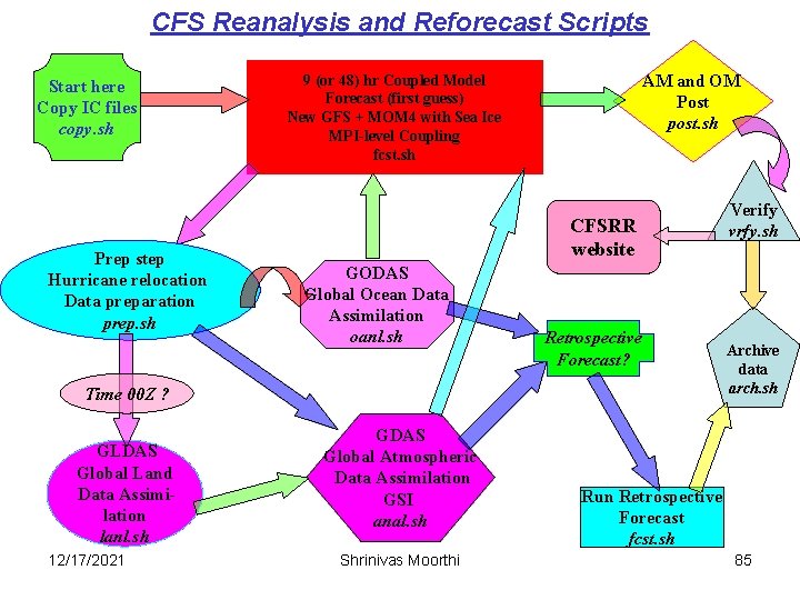
CFS Reanalysis and Reforecast Scripts Start here Copy IC files copy. sh Prep step Hurricane relocation Data preparation prep. sh AM and OM Post post. sh 9 (or 48) hr Coupled Model Forecast (first guess) New GFS + MOM 4 with Sea Ice MPI-level Coupling fcst. sh CFSRR website GODAS Global Ocean Data Assimilation oanl. sh Retrospective Forecast? Time 00 Z ? GLDAS Global Land Data Assimilation lanl. sh 12/17/2021 GDAS Global Atmospheric Data Assimilation GSI anal. sh Shrinivas Moorthi Verify vrfy. sh Archive data arch. sh Run Retrospective Forecast fcst. sh 85