Image Filtering and Edge Detection ECE 847 Digital

Image Filtering and Edge Detection ECE 847: Digital Image Processing Stan Birchfield Clemson University

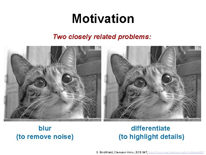
Motivation Two closely related problems: blur (to remove noise) differentiate (to highlight details) S. Birchfield, Clemson Univ. , ECE 847, http: //www. ces. clemson. edu/~stb/ece 847

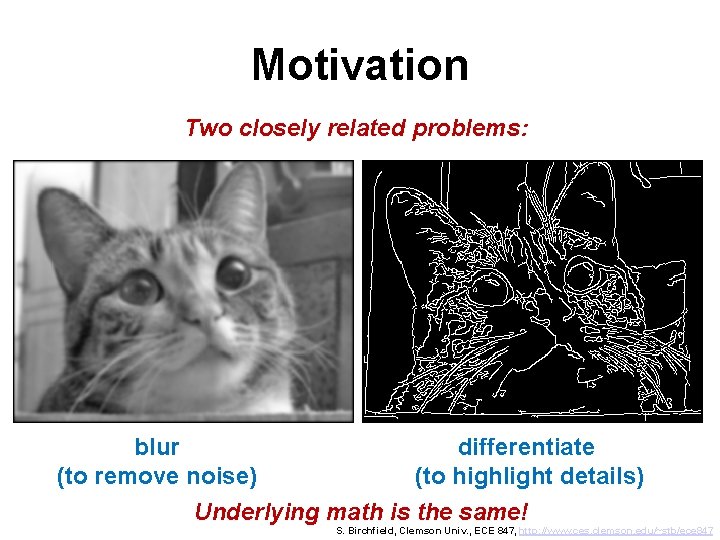
Motivation Two closely related problems: blur (to remove noise) differentiate (to highlight details) Underlying math is the same! S. Birchfield, Clemson Univ. , ECE 847, http: //www. ces. clemson. edu/~stb/ece 847

Recall: Types of image transformations • Graylevel transforms I’(x, y) f( I(x, y) ) (arithmetic, logical, thresholding, histogram equalization, …) • Geometric transforms I’(x, y) f( I(x’, y’) ) (flip, flop, rotate, scale, …) • Area-based transforms I’(x, y) f( I(x, y), I(x+1, y+1), … ) filtering (morphological operators, convolution) • Global transforms I’(x, y) f( I(x’, y’), x’, y’ ) (Fourier transform, wavelet transform) } A S. Birchfield, Clemson Univ. , ECE 847, http: //www. ces. clemson. edu/~stb/ece 847

Outline • • • Convolution Gaussian convolution kernels Smoothing an image Differentiating an image Canny edge detection Laplacian of Gaussian

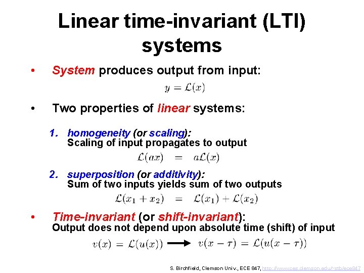
Linear time-invariant (LTI) systems • System produces output from input: • Two properties of linear systems: 1. homogeneity (or scaling): Scaling of input propagates to output 2. superposition (or additivity): Sum of two inputs yields sum of two outputs • Time-invariant (or shift-invariant): Output does not depend upon absolute time (shift) of input S. Birchfield, Clemson Univ. , ECE 847, http: //www. ces. clemson. edu/~stb/ece 847

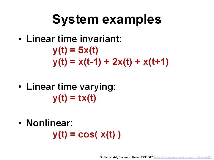
System examples • Linear time invariant: y(t) = 5 x(t) y(t) = x(t-1) + 2 x(t) + x(t+1) • Linear time varying: y(t) = tx(t) • Nonlinear: y(t) = cos( x(t) ) S. Birchfield, Clemson Univ. , ECE 847, http: //www. ces. clemson. edu/~stb/ece 847

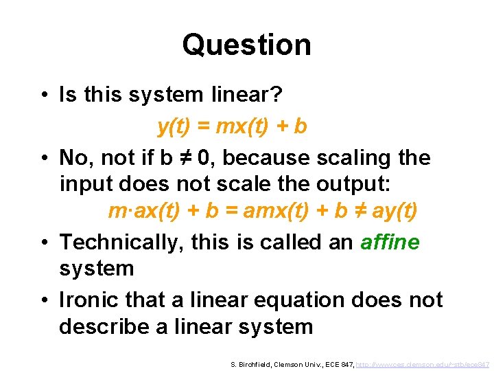
Question • Is this system linear? y(t) = mx(t) + b S. Birchfield, Clemson Univ. , ECE 847, http: //www. ces. clemson. edu/~stb/ece 847

Question • Is this system linear? y(t) = mx(t) + b • No, not if b ≠ 0, because scaling the input does not scale the output: m∙ax(t) + b = amx(t) + b ≠ ay(t) • Technically, this is called an affine system • Ironic that a linear equation does not describe a linear system S. Birchfield, Clemson Univ. , ECE 847, http: //www. ces. clemson. edu/~stb/ece 847

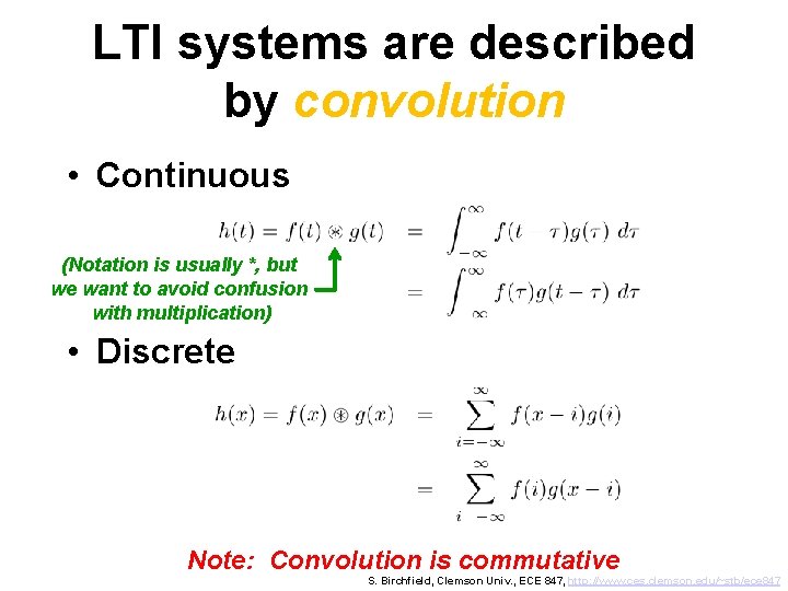
LTI systems are described by convolution • Continuous (Notation is usually *, but we want to avoid confusion with multiplication) • Discrete Note: Convolution is commutative S. Birchfield, Clemson Univ. , ECE 847, http: //www. ces. clemson. edu/~stb/ece 847

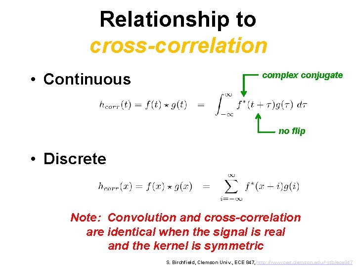
Relationship to cross-correlation • Continuous complex conjugate no flip • Discrete Note: Convolution and cross-correlation are identical when the signal is real and the kernel is symmetric S. Birchfield, Clemson Univ. , ECE 847, http: //www. ces. clemson. edu/~stb/ece 847

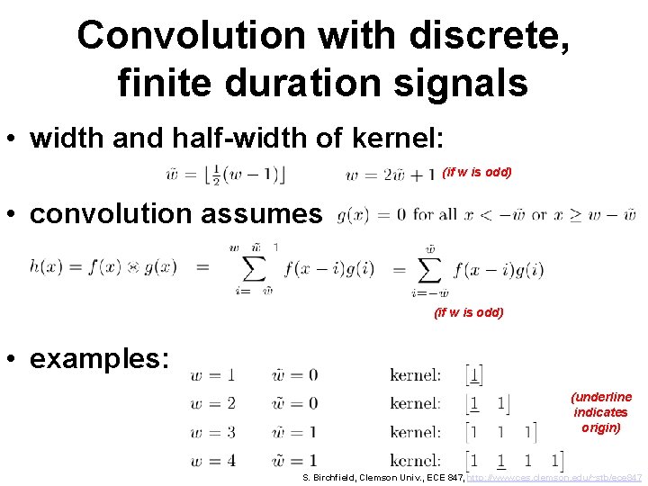
Convolution with discrete, finite duration signals • width and half-width of kernel: (if w is odd) • convolution assumes (if w is odd) • examples: (underline indicates origin) S. Birchfield, Clemson Univ. , ECE 847, http: //www. ces. clemson. edu/~stb/ece 847

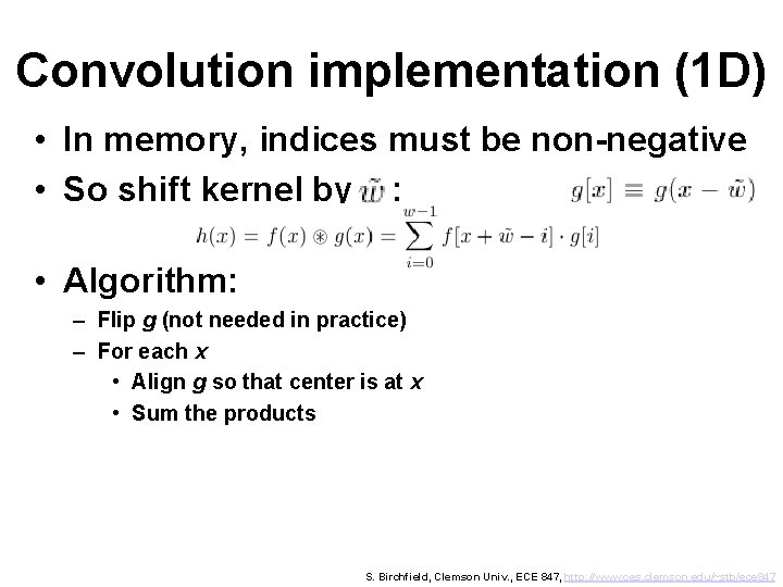
Convolution implementation (1 D) • In memory, indices must be non-negative • So shift kernel by : • Algorithm: – Flip g (not needed in practice) – For each x • Align g so that center is at x • Sum the products S. Birchfield, Clemson Univ. , ECE 847, http: //www. ces. clemson. edu/~stb/ece 847

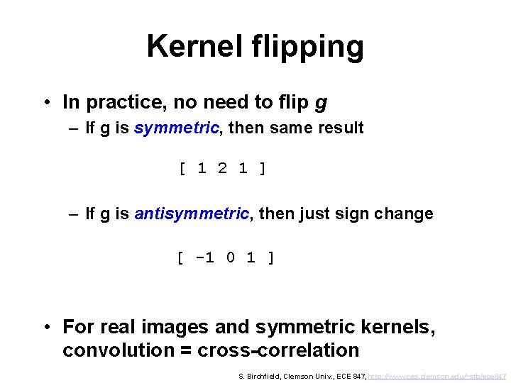
Kernel flipping • In practice, no need to flip g – If g is symmetric, then same result [ 1 2 1 ] – If g is antisymmetric, then just sign change [ -1 0 1 ] • For real images and symmetric kernels, convolution = cross-correlation S. Birchfield, Clemson Univ. , ECE 847, http: //www. ces. clemson. edu/~stb/ece 847

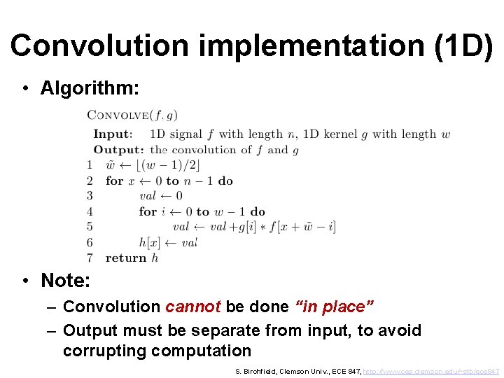
Convolution implementation (1 D) • Algorithm: • Note: – Convolution cannot be done “in place” – Output must be separate from input, to avoid corrupting computation S. Birchfield, Clemson Univ. , ECE 847, http: //www. ces. clemson. edu/~stb/ece 847

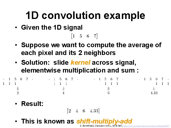
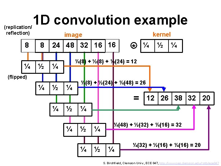
1 D convolution example • Given the 1 D signal • Suppose we want to compute the average of each pixel and its 2 neighbors • Solution: slide kernel across signal, elementwise multiplication and sum : • Result: • This is known as shift-multiply-add S. Birchfield, Clemson Univ. , ECE 847, http: //www. ces. clemson. edu/~stb/ece 847

Signal borders • Zero extension: [1 5 6 7] * [1/3 1/3] is the same as [… 0 1 5 6 7 0 …] * [… 0 1 1 1 0 …]/3 • Result: [… 0 0. 33 2 4 6 4. 33 2. 33 0 0 0 …] • If signal has length n and kernel has length w, then result has length n+w-1 • But we adopt convention of cropping output to same size as input S. Birchfield, Clemson Univ. , ECE 847, http: //www. ces. clemson. edu/~stb/ece 847

(replication/ reflection) 8 ¼ 1 D convolution example kernel image 8 ½ 24 48 32 16 16 ¼ ½ ½ ¼ ¼ ¼(8) + ½(24) + ¼(48) = 26 = ¼ ¼ ¼(8) + ½(8) + ¼(24) = 12 (flipped) ¼ * ½ ¼ 12 26 38 32 20 ¼ ½ ¼(48) + ½(32) + ¼(16) = 32 ¼ ¼(32) + ½(16) + ¼(16) = 20 S. Birchfield, Clemson Univ. , ECE 847, http: //www. ces. clemson. edu/~stb/ece 847

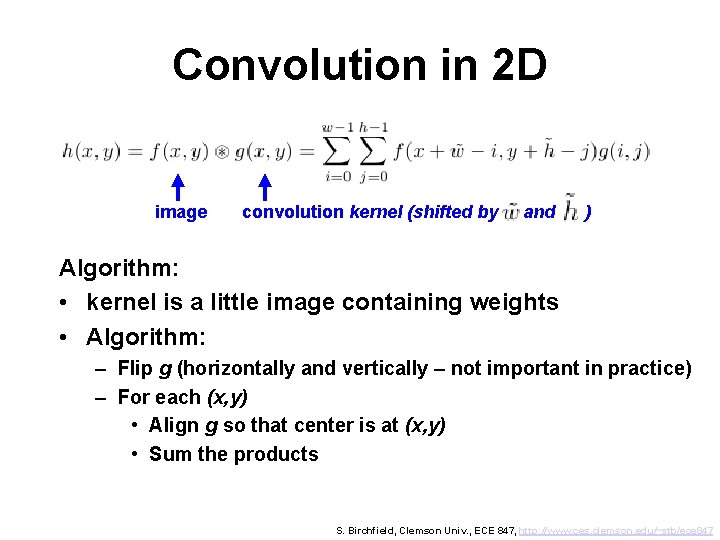
Convolution in 2 D image convolution kernel (shifted by and ) Algorithm: • kernel is a little image containing weights • Algorithm: – Flip g (horizontally and vertically – not important in practice) – For each (x, y) • Align g so that center is at (x, y) • Sum the products S. Birchfield, Clemson Univ. , ECE 847, http: //www. ces. clemson. edu/~stb/ece 847

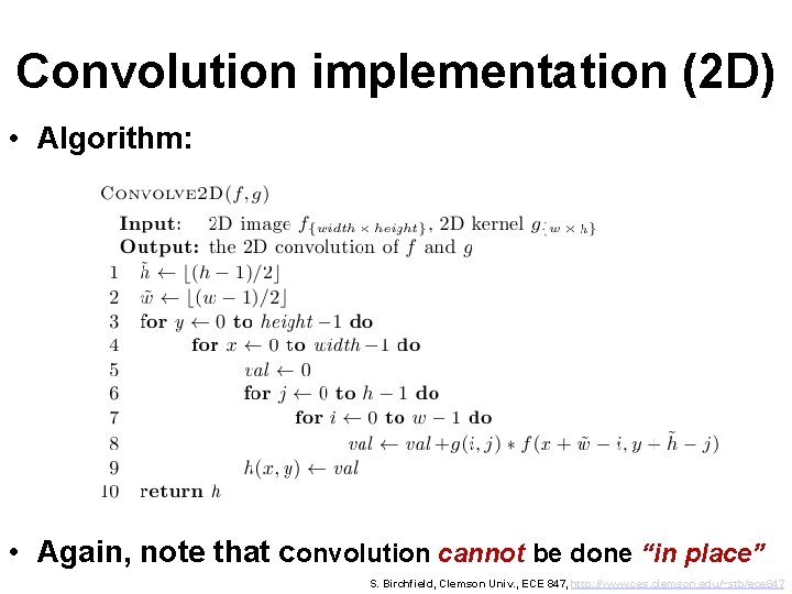
Convolution implementation (2 D) • Algorithm: • Again, note that convolution cannot be done “in place” S. Birchfield, Clemson Univ. , ECE 847, http: //www. ces. clemson. edu/~stb/ece 847

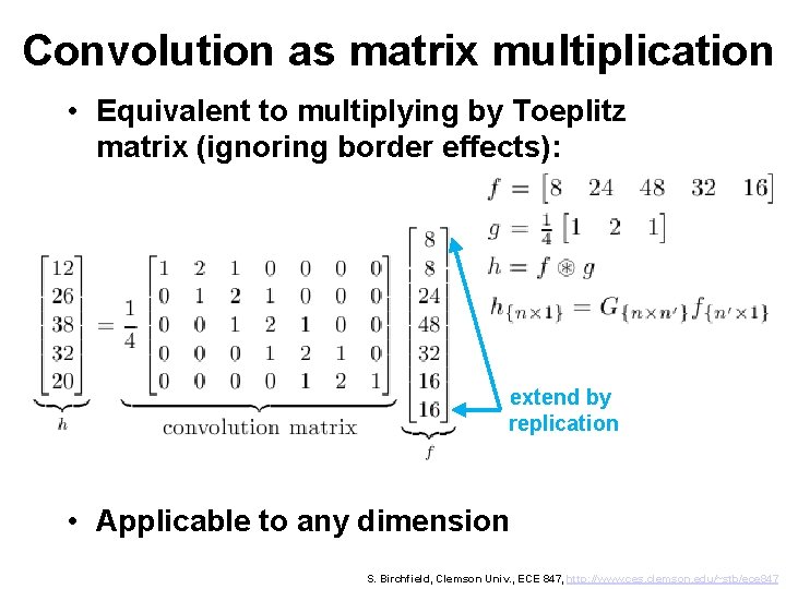
Convolution as matrix multiplication • Equivalent to multiplying by Toeplitz matrix (ignoring border effects): extend by replication • Applicable to any dimension S. Birchfield, Clemson Univ. , ECE 847, http: //www. ces. clemson. edu/~stb/ece 847

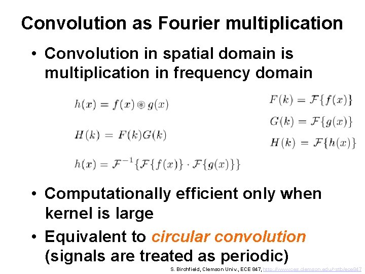
Convolution as Fourier multiplication • Convolution in spatial domain is multiplication in frequency domain • Computationally efficient only when kernel is large • Equivalent to circular convolution (signals are treated as periodic) S. Birchfield, Clemson Univ. , ECE 847, http: //www. ces. clemson. edu/~stb/ece 847

Outline • • • Convolution Gaussian convolution kernels Smoothing an image Differentiating an image Canny edge detection Laplacian of Gaussian

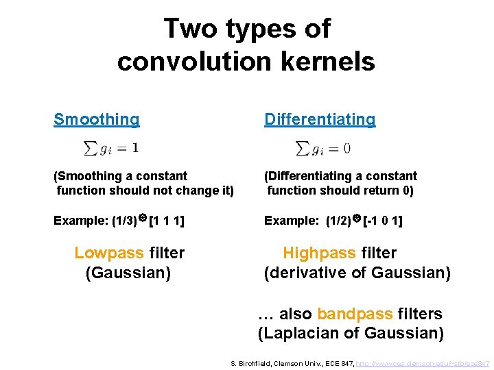
Two types of convolution kernels Smoothing Differentiating (Smoothing a constant function should not change it) (Differentiating a constant function should return 0) Example: (1/3) * [1 1 1] Example: (1/2) * [-1 0 1] Lowpass filter (Gaussian) Highpass filter (derivative of Gaussian) … also bandpass filters (Laplacian of Gaussian) S. Birchfield, Clemson Univ. , ECE 847, http: //www. ces. clemson. edu/~stb/ece 847

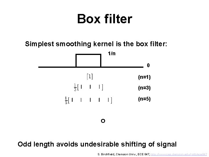
Box filter Simplest smoothing kernel is the box filter: 1/n 0 (n=1) (n=3) (n=5) Odd length avoids undesirable shifting of signal S. Birchfield, Clemson Univ. , ECE 847, http: //www. ces. clemson. edu/~stb/ece 847

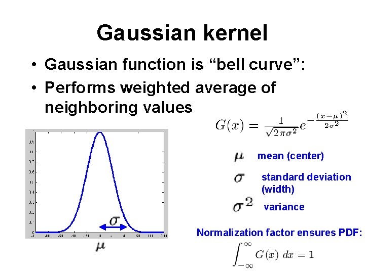
Gaussian kernel • Gaussian function is “bell curve”: • Performs weighted average of neighboring values mean (center) standard deviation (width) variance Normalization factor ensures PDF:

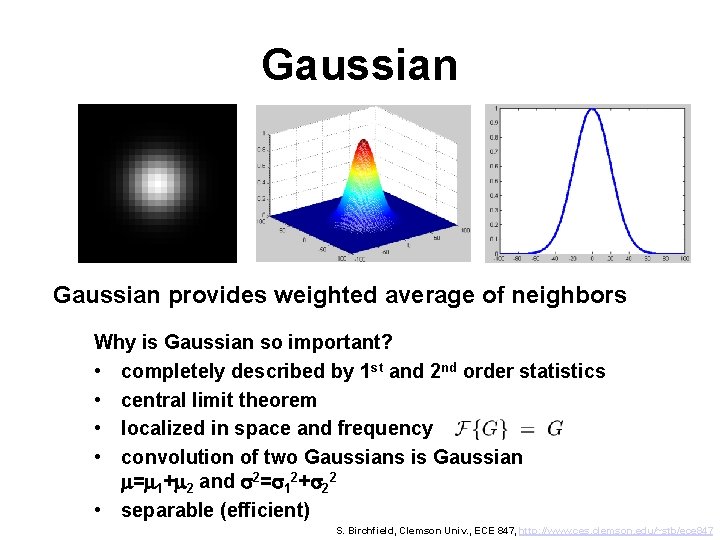
Gaussian provides weighted average of neighbors Why is Gaussian so important? • completely described by 1 st and 2 nd order statistics • central limit theorem • localized in space and frequency • convolution of two Gaussians is Gaussian m=m 1+m 2 and s 2=s 12+s 22 • separable (efficient) S. Birchfield, Clemson Univ. , ECE 847, http: //www. ces. clemson. edu/~stb/ece 847

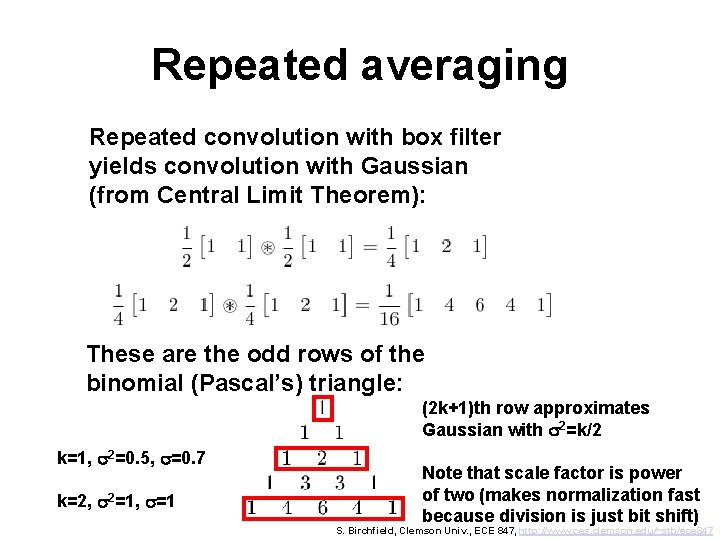
Repeated averaging Repeated convolution with box filter yields convolution with Gaussian (from Central Limit Theorem): These are the odd rows of the binomial (Pascal’s) triangle: (2 k+1)th row approximates Gaussian with s 2=k/2 k=1, s 2=0. 5, s=0. 7 k=2, s 2=1, s=1 Note that scale factor is power of two (makes normalization fast because division is just bit shift) S. Birchfield, Clemson Univ. , ECE 847, http: //www. ces. clemson. edu/~stb/ece 847

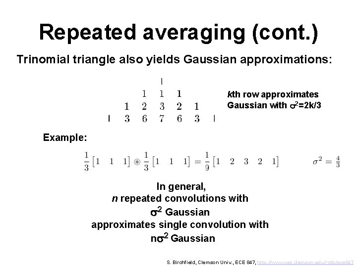
Repeated averaging (cont. ) Trinomial triangle also yields Gaussian approximations: kth row approximates Gaussian with s 2=2 k/3 Example: In general, n repeated convolutions with s 2 Gaussian approximates single convolution with ns 2 Gaussian S. Birchfield, Clemson Univ. , ECE 847, http: //www. ces. clemson. edu/~stb/ece 847

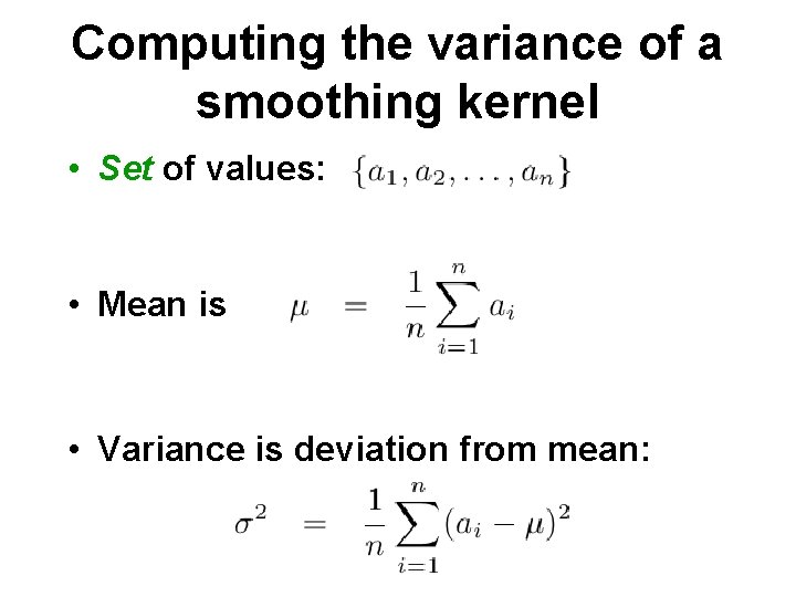
Computing the variance of a smoothing kernel • Set of values: • Mean is • Variance is deviation from mean:

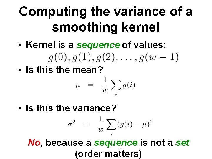
Computing the variance of a smoothing kernel • Kernel is a sequence of values: • Is this the mean? • Is this the variance? No, because a sequence is not a set (order matters)

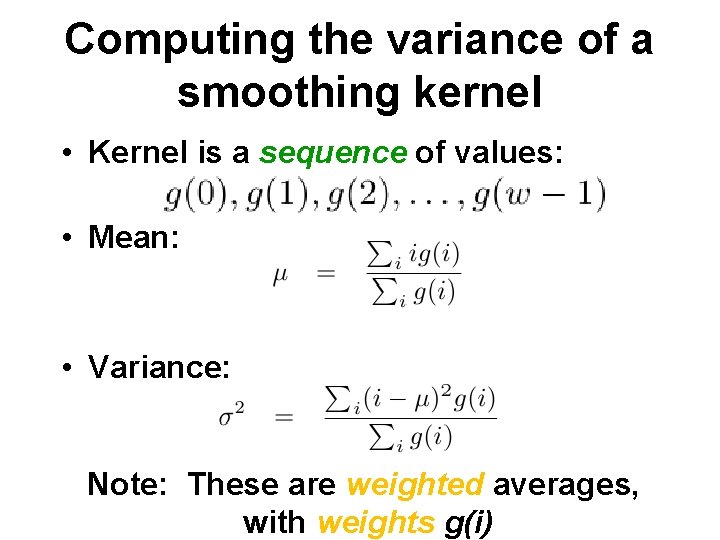
Computing the variance of a smoothing kernel • Kernel is a sequence of values: • Mean: • Variance: Note: These are weighted averages, with weights g(i)

Example • Kernel: g[0] g[1] g[2] • Mean: • Variance: 2 1 1 0 1 2 Note:

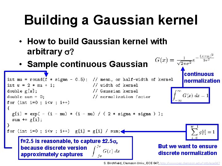
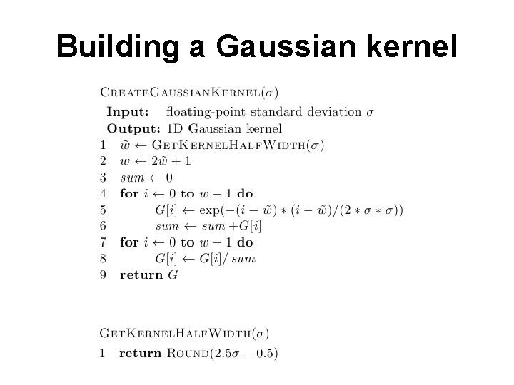
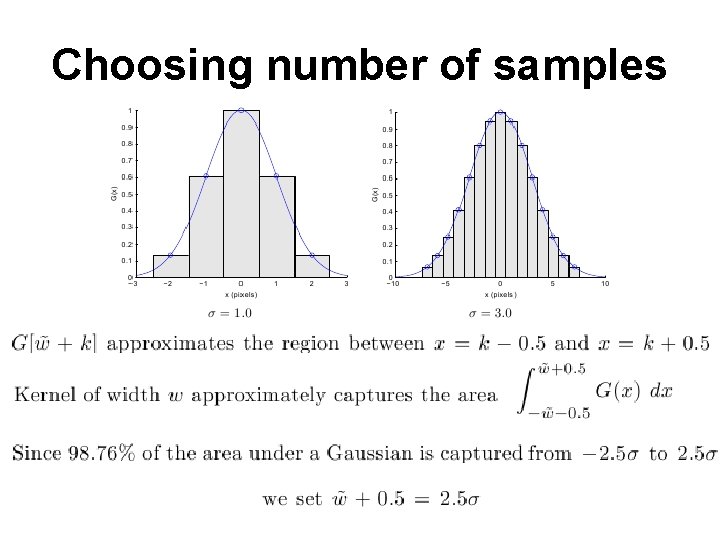
Building a Gaussian kernel • How to build Gaussian kernel with arbitrary s? • Sample continuous Gaussian continuous normalization f=2. 5 is reasonable, to capture ± 2. 5 s, because discrete version approximately captures But we want to ensure discrete normalization S. Birchfield, Clemson Univ. , ECE 847, http: //www. ces. clemson. edu/~stb/ece 847

Building a Gaussian kernel

Choosing number of samples

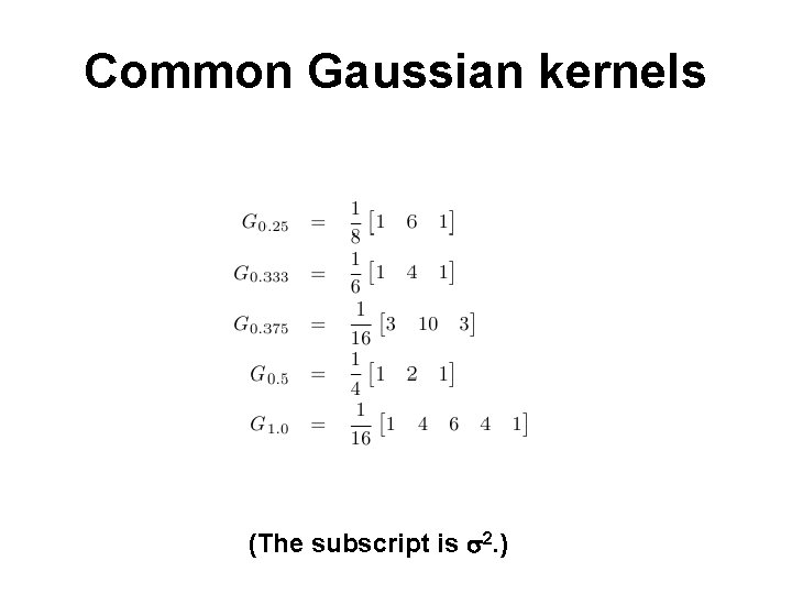
Common Gaussian kernels (The subscript is s 2. )

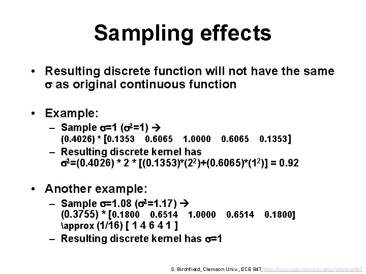
Sampling effects • Resulting discrete function will not have the same s as original continuous function • Example: – Sample s=1 (s 2=1) (0. 4026) * [0. 1353 0. 6065 1. 0000 0. 6065 0. 1353] – Resulting discrete kernel has s 2=(0. 4026) * 2 * [(0. 1353)*(22)+(0. 6065)*(12)] = 0. 92 • Another example: – Sample s=1. 08 (s 2=1. 17) (0. 3755) * [0. 1800 0. 6514 1. 0000 0. 6514 0. 1800] approx (1/16) [ 1 4 6 4 1 ] – Resulting discrete kernel has s=1 S. Birchfield, Clemson Univ. , ECE 847, http: //www. ces. clemson. edu/~stb/ece 847

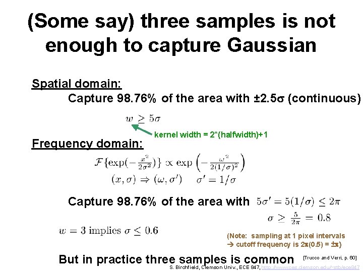
(Some say) three samples is not enough to capture Gaussian Spatial domain: Capture 98. 76% of the area with ± 2. 5 s (continuous) Frequency domain: kernel width = 2*(halfwidth)+1 Capture 98. 76% of the area with (Note: sampling at 1 pixel intervals cutoff frequency is 2 p(0. 5) = ±p) [Trucco and Verri, p. 60] But in practice three samples is common S. Birchfield, Clemson Univ. , ECE 847, http: //www. ces. clemson. edu/~stb/ece 847

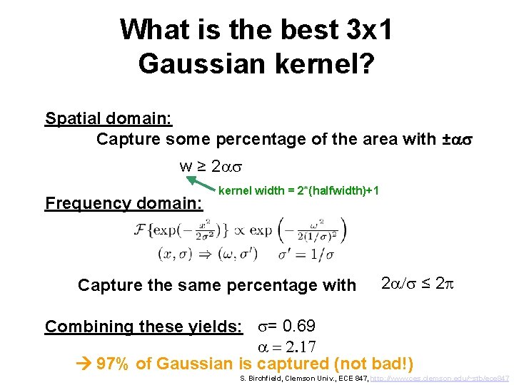
What is the best 3 x 1 Gaussian kernel? Spatial domain: Capture some percentage of the area with ±as w ≥ 2 as Frequency domain: kernel width = 2*(halfwidth)+1 Capture the same percentage with 2 a/s ≤ 2 p Combining these yields: s= 0. 69 a = 2. 17 97% of Gaussian is captured (not bad!) S. Birchfield, Clemson Univ. , ECE 847, http: //www. ces. clemson. edu/~stb/ece 847

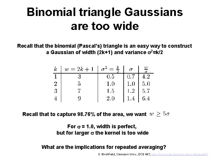
Binomial triangle Gaussians are too wide Recall that the binomial (Pascal’s) triangle is an easy way to construct a Gaussian of width (2 k+1) and variance s 2=k/2 Recall that to capture 98. 76% of the area, we want For s = 1. 0, width is perfect, but for larger s the kernel is too wide What are the implications for repeated averaging? S. Birchfield, Clemson Univ. , ECE 847, http: //www. ces. clemson. edu/~stb/ece 847

Outline • • • Convolution Gaussian convolution kernels Smoothing an image Differentiating an image Canny edge detection Laplacian of Gaussian

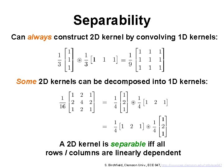
Separability Can always construct 2 D kernel by convolving 1 D kernels: Some 2 D kernels can be decomposed into 1 D kernels: A 2 D kernel is separable iff all rows / columns are linearly dependent S. Birchfield, Clemson Univ. , ECE 847, http: //www. ces. clemson. edu/~stb/ece 847

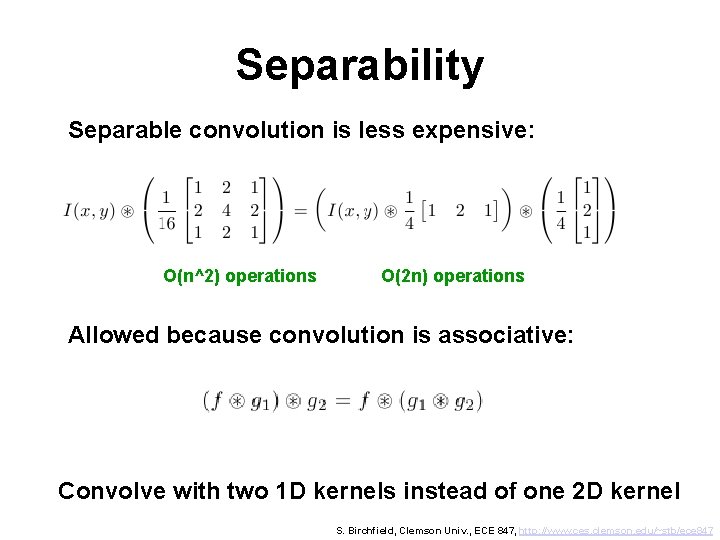
Separability Separable convolution is less expensive: O(n^2) operations O(2 n) operations Allowed because convolution is associative: Convolve with two 1 D kernels instead of one 2 D kernel S. Birchfield, Clemson Univ. , ECE 847, http: //www. ces. clemson. edu/~stb/ece 847

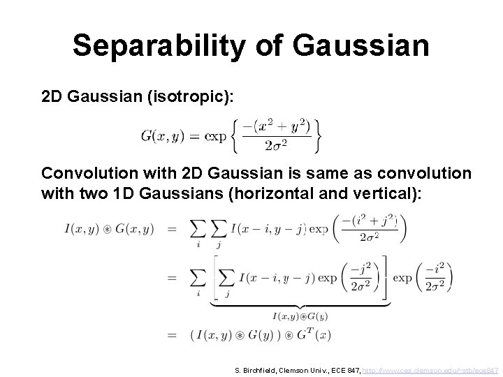
Separability of Gaussian 2 D Gaussian (isotropic): Convolution with 2 D Gaussian is same as convolution with two 1 D Gaussians (horizontal and vertical): S. Birchfield, Clemson Univ. , ECE 847, http: //www. ces. clemson. edu/~stb/ece 847

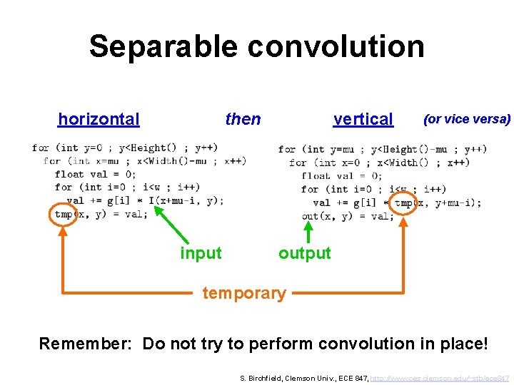
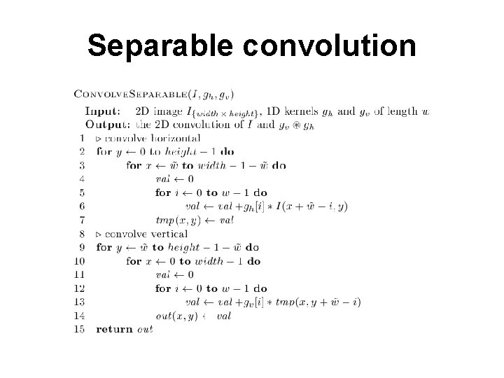
Separable convolution horizontal then input vertical (or vice versa) output temporary Remember: Do not try to perform convolution in place! S. Birchfield, Clemson Univ. , ECE 847, http: //www. ces. clemson. edu/~stb/ece 847

Separable convolution

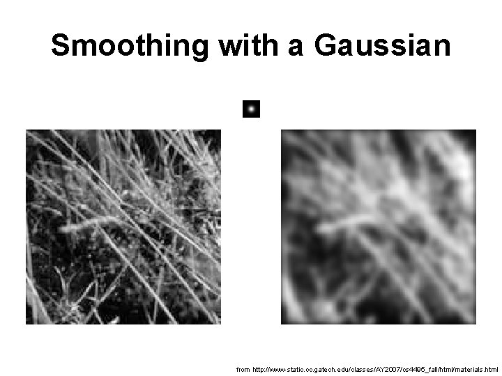
Smoothing with a Gaussian from http: //www-static. cc. gatech. edu/classes/AY 2007/cs 4495_fall/html/materials. html

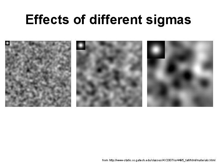
Effects of different sigmas from http: //www-static. cc. gatech. edu/classes/AY 2007/cs 4495_fall/html/materials. html

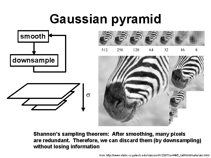
Gaussian pyramid smooth downsample s Shannon’s sampling theorem: After smoothing, many pixels are redundant. Therefore, we can discard them (by downsampling) without losing information from http: //www-static. cc. gatech. edu/classes/AY 2007/cs 4495_fall/html/materials. html

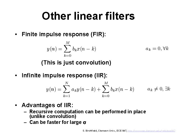
Other linear filters • Finite impulse response (FIR): (This is just convolution) • Infinite impulse response (IIR): • Advantages of IIR: – Recursive computation can be performed in place (unlike convolution) – Can be faster for large s S. Birchfield, Clemson Univ. , ECE 847, http: //www. ces. clemson. edu/~stb/ece 847

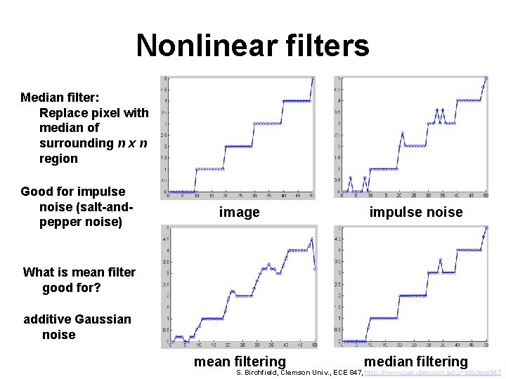
Nonlinear filters Median filter: Replace pixel with median of surrounding n x n region Good for impulse noise (salt-andpepper noise) image impulse noise mean filtering median filtering What is mean filter good for? additive Gaussian noise S. Birchfield, Clemson Univ. , ECE 847, http: //www. ces. clemson. edu/~stb/ece 847

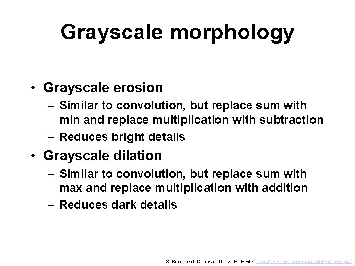
Grayscale morphology • Grayscale erosion – Similar to convolution, but replace sum with min and replace multiplication with subtraction – Reduces bright details • Grayscale dilation – Similar to convolution, but replace sum with max and replace multiplication with addition – Reduces dark details S. Birchfield, Clemson Univ. , ECE 847, http: //www. ces. clemson. edu/~stb/ece 847

Outline • • • Convolution Gaussian convolution kernels Smoothing an image Differentiating an image Canny edge detection Laplacian of Gaussian

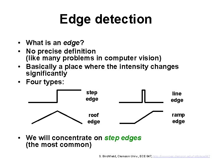
Edge detection • What is an edge? • No precise definition (like many problems in computer vision) • Basically a place where the intensity changes significantly • Four types: step edge line edge roof edge ramp edge • We will concentrate on step edges (the most common) S. Birchfield, Clemson Univ. , ECE 847, http: //www. ces. clemson. edu/~stb/ece 847

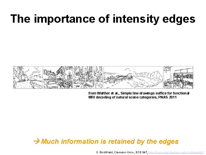
The importance of intensity edges from Walther et al. , Simple line drawings suffice for functional MRI decoding of natural scene categories, PNAS 2011 Much information is retained by the edges S. Birchfield, Clemson Univ. , ECE 847, http: //www. ces. clemson. edu/~stb/ece 847

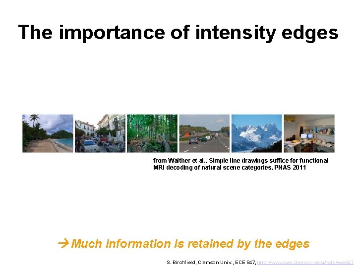
The importance of intensity edges from Walther et al. , Simple line drawings suffice for functional MRI decoding of natural scene categories, PNAS 2011 Much information is retained by the edges S. Birchfield, Clemson Univ. , ECE 847, http: //www. ces. clemson. edu/~stb/ece 847

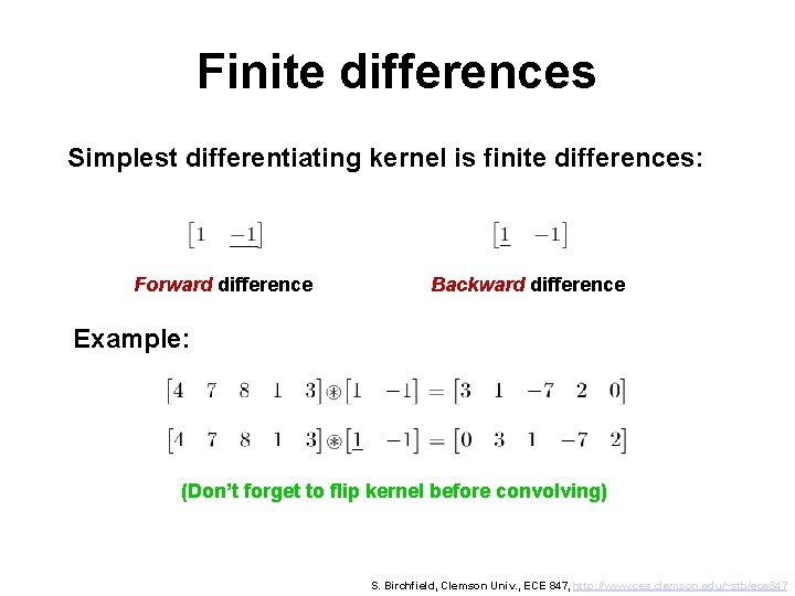
Finite differences Simplest differentiating kernel is finite differences: Forward difference Backward difference Example: (Don’t forget to flip kernel before convolving) S. Birchfield, Clemson Univ. , ECE 847, http: //www. ces. clemson. edu/~stb/ece 847

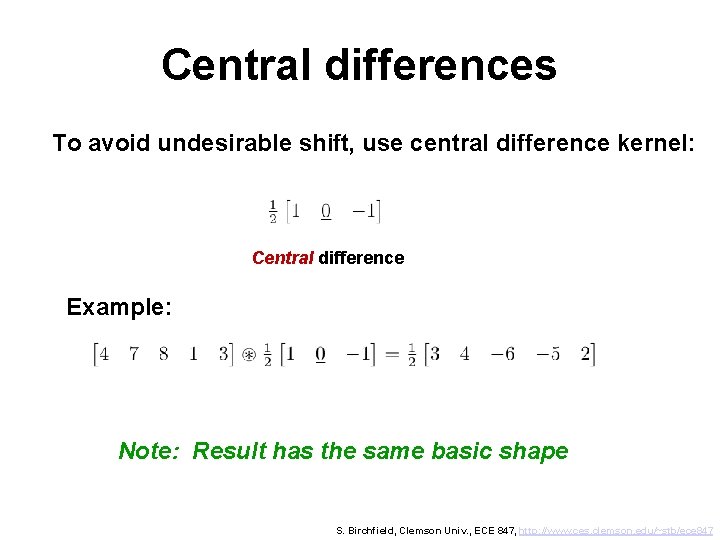
Central differences To avoid undesirable shift, use central difference kernel: Central difference Example: Note: Result has the same basic shape S. Birchfield, Clemson Univ. , ECE 847, http: //www. ces. clemson. edu/~stb/ece 847

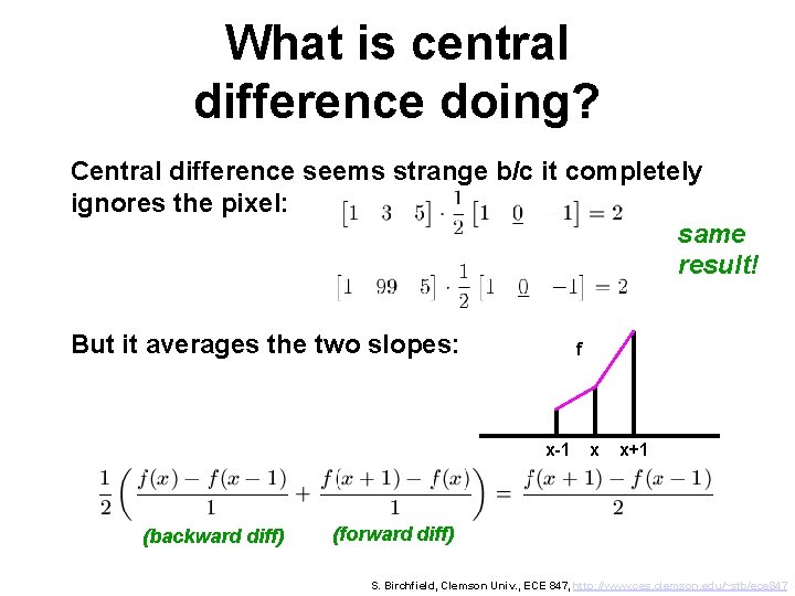
What is central difference doing? Central difference seems strange b/c it completely ignores the pixel: same result! But it averages the two slopes: f x-1 (backward diff) x x+1 (forward diff) S. Birchfield, Clemson Univ. , ECE 847, http: //www. ces. clemson. edu/~stb/ece 847

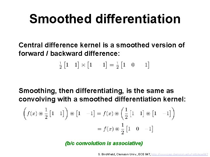
Smoothed differentiation Central difference kernel is a smoothed version of forward / backward difference: Smoothing, then differentiating, is the same as convolving with a smoothed differentiation kernel: (b/c convolution is associative) S. Birchfield, Clemson Univ. , ECE 847, http: //www. ces. clemson. edu/~stb/ece 847

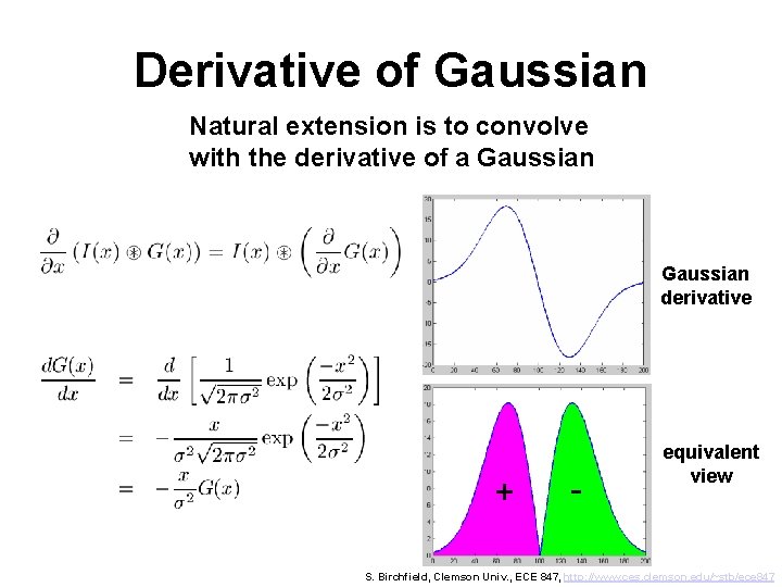
Derivative of Gaussian Natural extension is to convolve with the derivative of a Gaussian derivative + - equivalent view S. Birchfield, Clemson Univ. , ECE 847, http: //www. ces. clemson. edu/~stb/ece 847

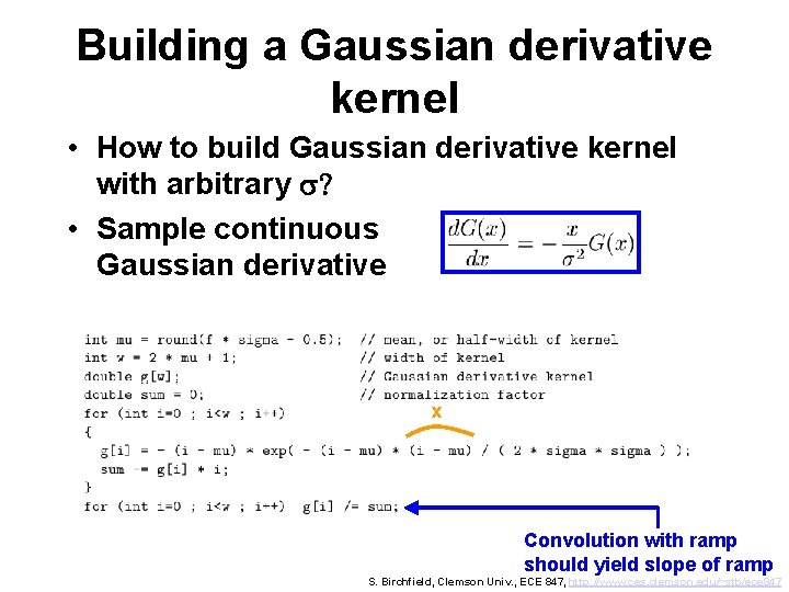
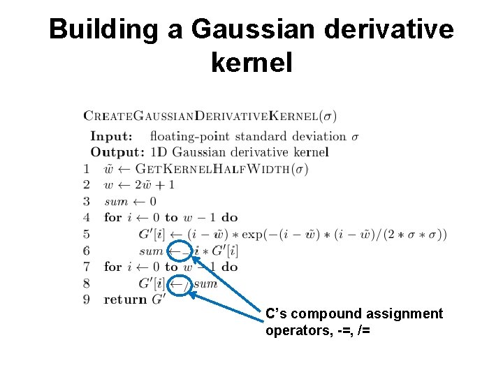
Building a Gaussian derivative kernel • How to build Gaussian derivative kernel with arbitrary s? • Sample continuous Gaussian derivative x Convolution with ramp should yield slope of ramp S. Birchfield, Clemson Univ. , ECE 847, http: //www. ces. clemson. edu/~stb/ece 847

Building a Gaussian derivative kernel C’s compound assignment operators, -=, /=

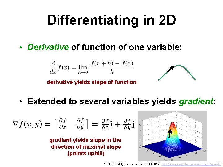
Differentiating in 2 D • Derivative of function of one variable: derivative yields slope of function • Extended to several variables yields gradient: gradient yields slope in the direction of maximal slope (points uphill) S. Birchfield, Clemson Univ. , ECE 847, http: //www. ces. clemson. edu/~stb/ece 847

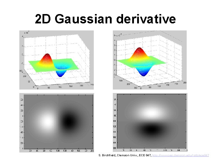
2 D Gaussian derivative S. Birchfield, Clemson Univ. , ECE 847, http: //www. ces. clemson. edu/~stb/ece 847

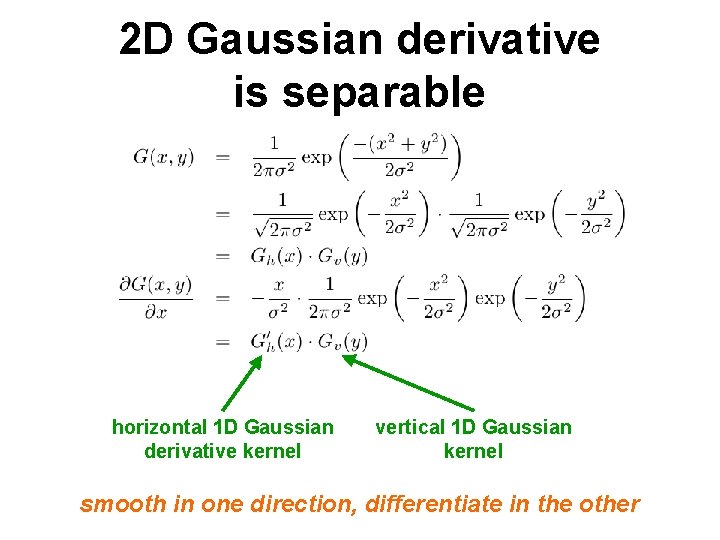
2 D Gaussian derivative is separable horizontal 1 D Gaussian derivative kernel vertical 1 D Gaussian kernel smooth in one direction, differentiate in the other

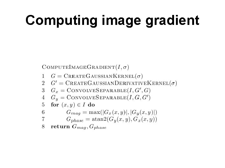
Computing image gradient

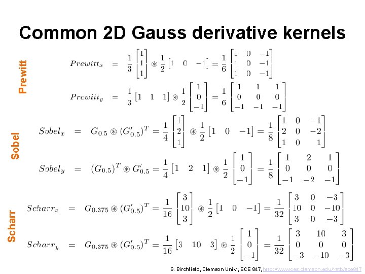
Scharr Sobel Prewitt Common 2 D Gauss derivative kernels S. Birchfield, Clemson Univ. , ECE 847, http: //www. ces. clemson. edu/~stb/ece 847

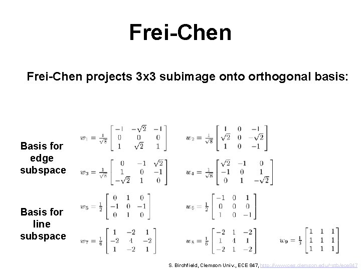
Frei-Chen projects 3 x 3 subimage onto orthogonal basis: Basis for edge subspace Basis for line subspace S. Birchfield, Clemson Univ. , ECE 847, http: //www. ces. clemson. edu/~stb/ece 847

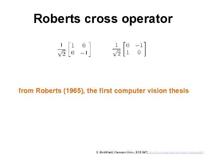
Roberts cross operator from Roberts (1965), the first computer vision thesis S. Birchfield, Clemson Univ. , ECE 847, http: //www. ces. clemson. edu/~stb/ece 847

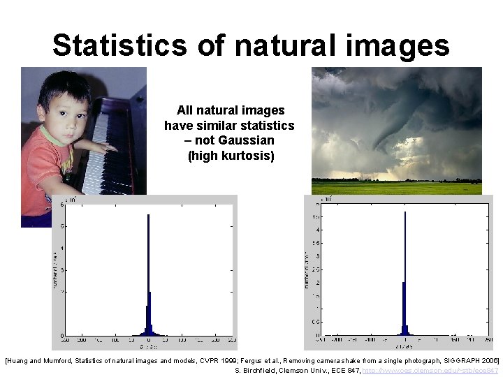
Statistics of natural images All natural images have similar statistics – not Gaussian (high kurtosis) [Huang and Mumford, Statistics of natural images and models, CVPR 1999; Fergus et al. , Removing camera shake from a single photograph, SIGGRAPH 2006] S. Birchfield, Clemson Univ. , ECE 847, http: //www. ces. clemson. edu/~stb/ece 847

Outline • • • Convolution Gaussian convolution kernels Smoothing an image Differentiating an image Canny edge detection Laplacian of Gaussian

Canny edge detection • Landmark paper (1986) • Key ideas: – – – theoretical basis for Gaussian derivative non-maximal suppression edge following hysteresis (double thresholding) feature synthesis (early version of scale space) • Still popular because – – easy to implement small number of intuitive parameters computationally efficient good results S. Birchfield, Clemson Univ. , ECE 847, http: //www. ces. clemson. edu/~stb/ece 847

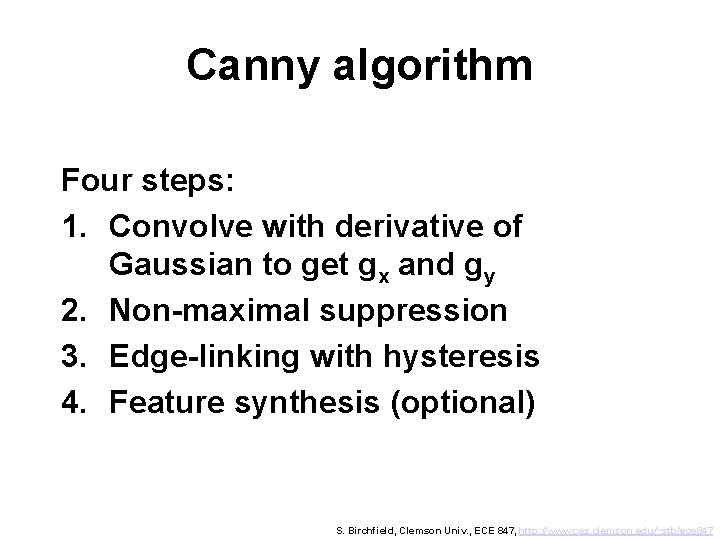
Canny algorithm Four steps: 1. Convolve with derivative of Gaussian to get gx and gy 2. Non-maximal suppression 3. Edge-linking with hysteresis 4. Feature synthesis (optional) S. Birchfield, Clemson Univ. , ECE 847, http: //www. ces. clemson. edu/~stb/ece 847

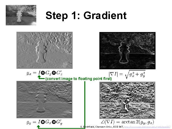
Step 1: Gradient (convert image to floating point first) S. Birchfield, Clemson Univ. , ECE 847, http: //www. ces. clemson. edu/~stb/ece 847

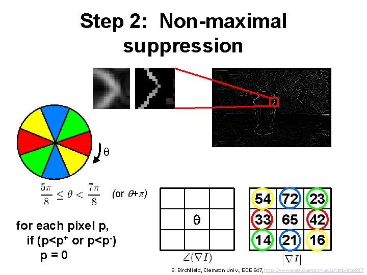
Step 2: Non-maximal suppression q (or q+p) for each pixel p, if (p<p+ or p<p-) p=0 q 54 72 23 33 65 42 14 21 16 S. Birchfield, Clemson Univ. , ECE 847, http: //www. ces. clemson. edu/~stb/ece 847

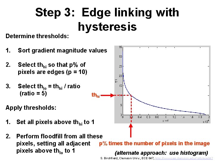
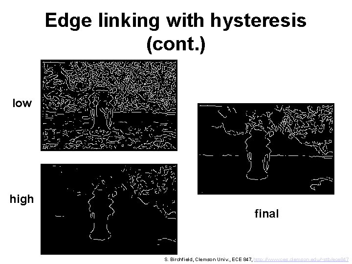
Step 3: Edge linking with hysteresis Determine thresholds: 1. Sort gradient magnitude values 2. Select thhi so that p% of pixels are edges (p = 10) 3. Select thlo = thhi / ratio (ratio = 5) thhi Apply thresholds: 1. Set all pixels above thhi to 1 2. Perform floodfill from all these pixels, setting all adjacent p% times the number of pixels in the image pixels above thlo to 1 (alternate approach: use histogram) S. Birchfield, Clemson Univ. , ECE 847, http: //www. ces. clemson. edu/~stb/ece 847

Edge linking with hysteresis (cont. ) low high final S. Birchfield, Clemson Univ. , ECE 847, http: //www. ces. clemson. edu/~stb/ece 847

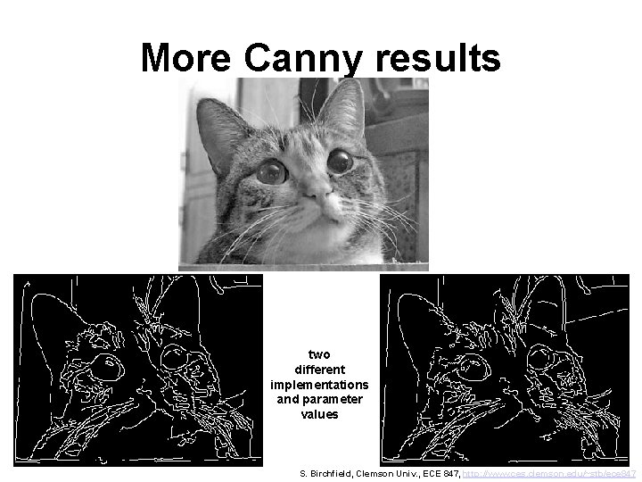
More Canny results two different implementations and parameter values S. Birchfield, Clemson Univ. , ECE 847, http: //www. ces. clemson. edu/~stb/ece 847

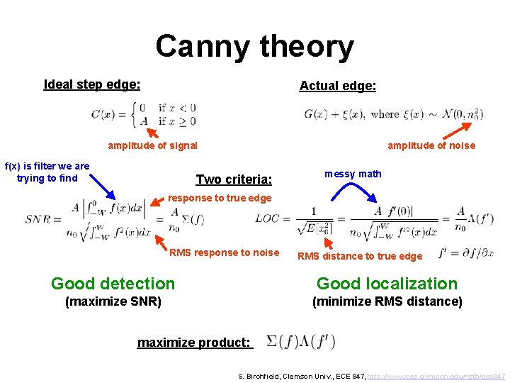
Canny theory Ideal step edge: Actual edge: amplitude of signal f(x) is filter we are trying to find amplitude of noise Two criteria: messy math response to true edge RMS response to noise RMS distance to true edge Good detection Good localization (maximize SNR) (minimize RMS distance) maximize product: S. Birchfield, Clemson Univ. , ECE 847, http: //www. ces. clemson. edu/~stb/ece 847

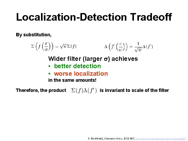
Localization-Detection Tradeoff By substitution, Wider filter (larger s) achieves • better detection • worse localization in the same amounts! Therefore, the product is invariant to scale of the filter S. Birchfield, Clemson Univ. , ECE 847, http: //www. ces. clemson. edu/~stb/ece 847

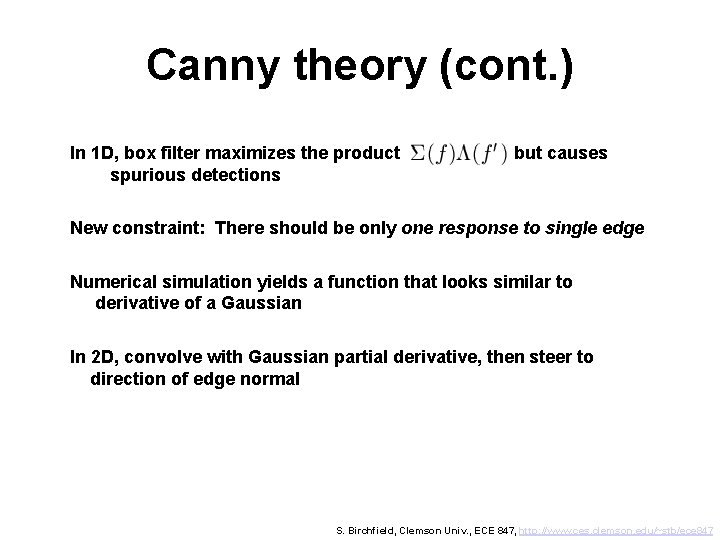
Canny theory (cont. ) In 1 D, box filter maximizes the product spurious detections but causes New constraint: There should be only one response to single edge Numerical simulation yields a function that looks similar to derivative of a Gaussian In 2 D, convolve with Gaussian partial derivative, then steer to direction of edge normal S. Birchfield, Clemson Univ. , ECE 847, http: //www. ces. clemson. edu/~stb/ece 847

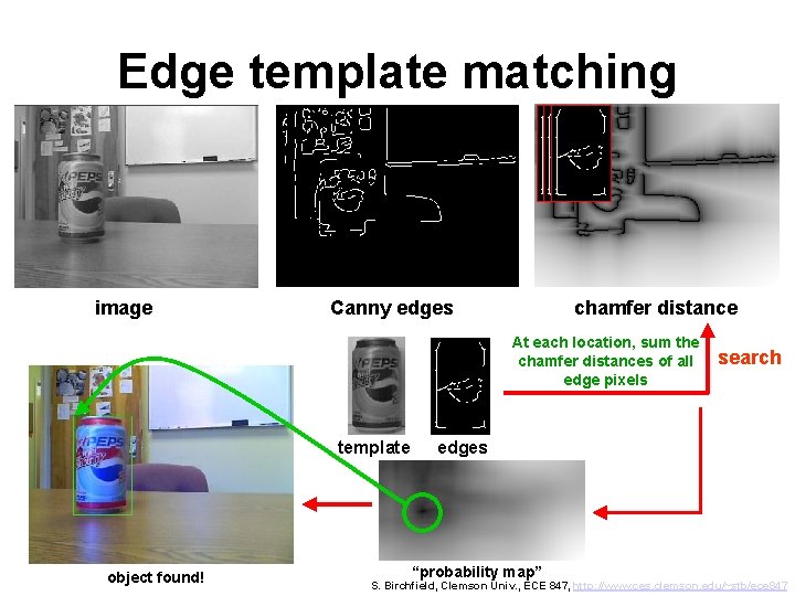
Edge template matching image Canny edges chamfer distance At each location, sum the chamfer distances of all edge pixels template object found! search edges “probability map” S. Birchfield, Clemson Univ. , ECE 847, http: //www. ces. clemson. edu/~stb/ece 847

Outline • • • Convolution Gaussian convolution kernels Smoothing an image Differentiating an image Canny edge detection Laplacian of Gaussian

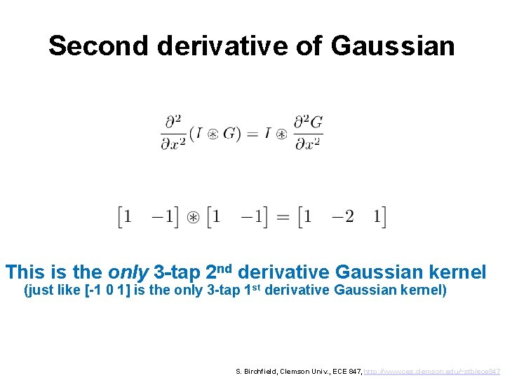
Second derivative of Gaussian This is the only 3 -tap 2 nd derivative Gaussian kernel (just like [-1 0 1] is the only 3 -tap 1 st derivative Gaussian kernel) S. Birchfield, Clemson Univ. , ECE 847, http: //www. ces. clemson. edu/~stb/ece 847

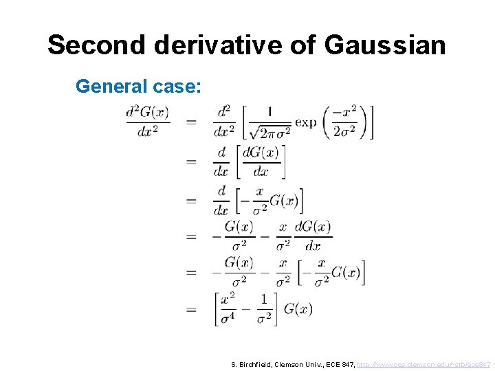
Second derivative of Gaussian General case: S. Birchfield, Clemson Univ. , ECE 847, http: //www. ces. clemson. edu/~stb/ece 847

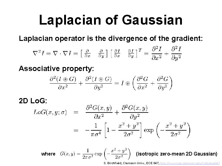
Laplacian of Gaussian Laplacian operator is the divergence of the gradient: Associative property: 2 D Lo. G: where (isotropic zero-mean 2 D Gaussian) S. Birchfield, Clemson Univ. , ECE 847, http: //www. ces. clemson. edu/~stb/ece 847

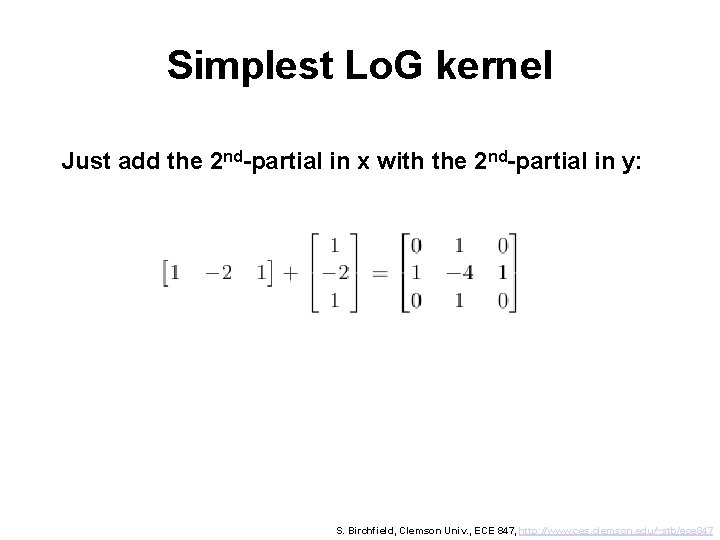
Simplest Lo. G kernel Just add the 2 nd-partial in x with the 2 nd-partial in y: S. Birchfield, Clemson Univ. , ECE 847, http: //www. ces. clemson. edu/~stb/ece 847

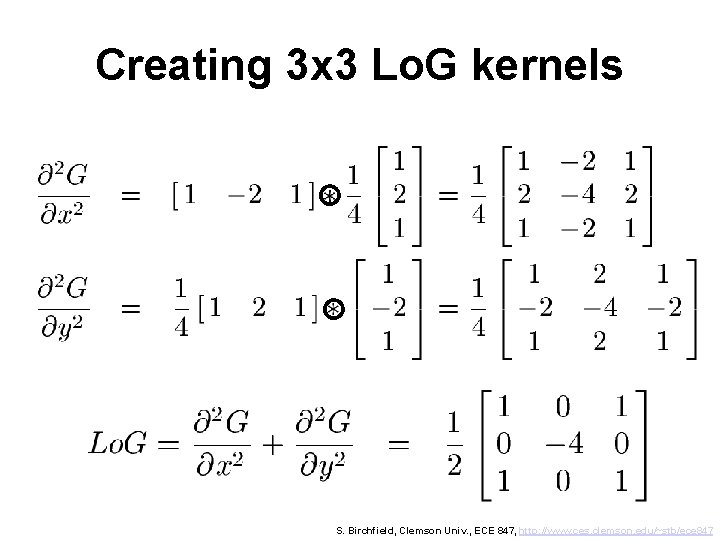
Creating 3 x 3 Lo. G kernels S. Birchfield, Clemson Univ. , ECE 847, http: //www. ces. clemson. edu/~stb/ece 847

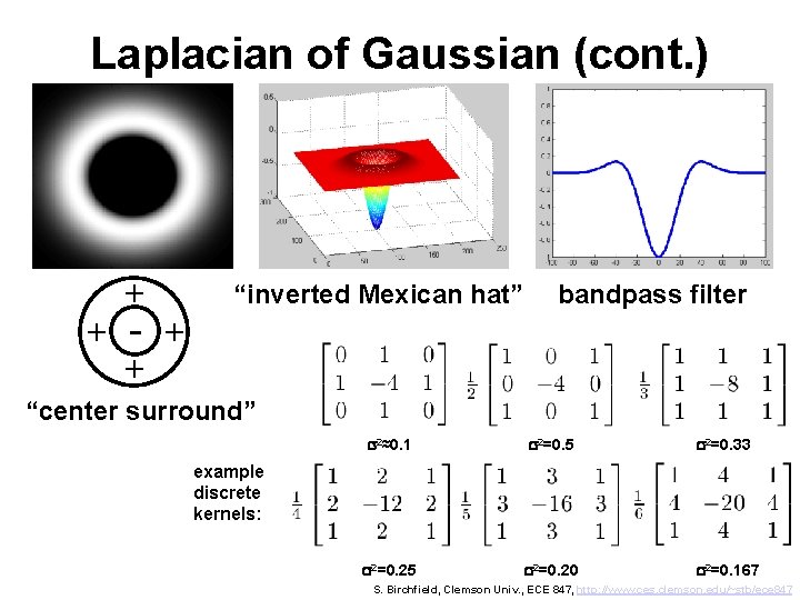
Laplacian of Gaussian (cont. ) + + - + + “inverted Mexican hat” bandpass filter “center surround” s 2≈0. 1 s 2=0. 5 s 2=0. 33 s 2=0. 25 s 2=0. 20 s 2=0. 167 example discrete kernels: S. Birchfield, Clemson Univ. , ECE 847, http: //www. ces. clemson. edu/~stb/ece 847

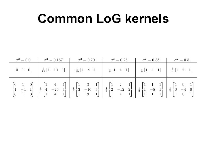
Common Lo. G kernels

Marr-Hildreth operator • Marr-Hildreth (1980) • Zero crossings of 2 nd derivative are extrema of 1 st derivative • Center surround, biologically plausible (difference of Gaussian) • Not separable (but sum of two kernels, each of which is separable) • Not as good as Canny, b/c smooths across boundary • Generates closed curves S. Birchfield, Clemson Univ. , ECE 847, http: //www. ces. clemson. edu/~stb/ece 847

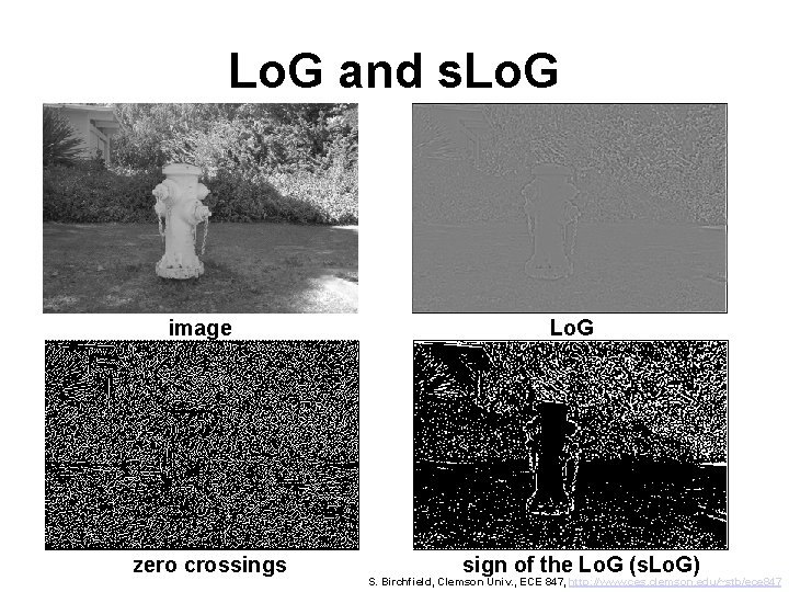
Lo. G and s. Lo. G image zero crossings Lo. G sign of the Lo. G (s. Lo. G) S. Birchfield, Clemson Univ. , ECE 847, http: //www. ces. clemson. edu/~stb/ece 847

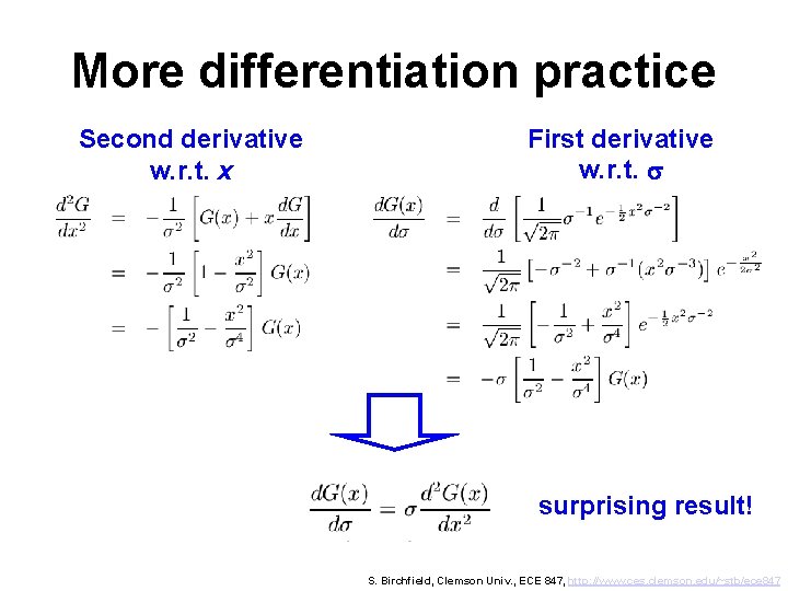
More differentiation practice Second derivative w. r. t. x First derivative w. r. t. s surprising result! S. Birchfield, Clemson Univ. , ECE 847, http: //www. ces. clemson. edu/~stb/ece 847

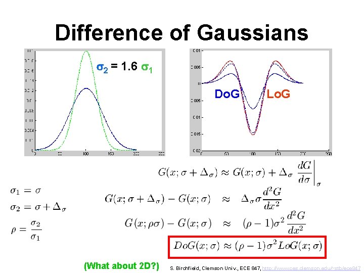
Difference of Gaussians s 2 = 1. 6 s 1 Do. G (What about 2 D? ) Lo. G S. Birchfield, Clemson Univ. , ECE 847, http: //www. ces. clemson. edu/~stb/ece 847

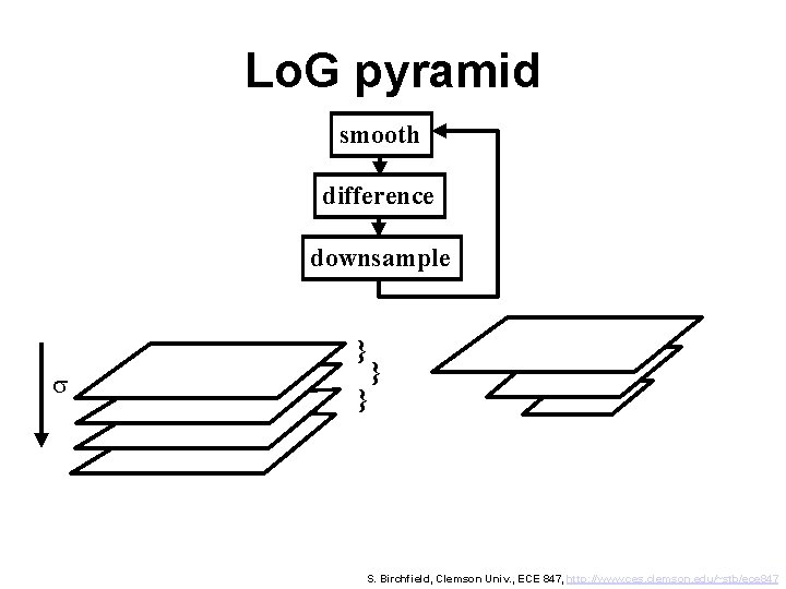
Lo. G pyramid smooth difference downsample } s } } S. Birchfield, Clemson Univ. , ECE 847, http: //www. ces. clemson. edu/~stb/ece 847

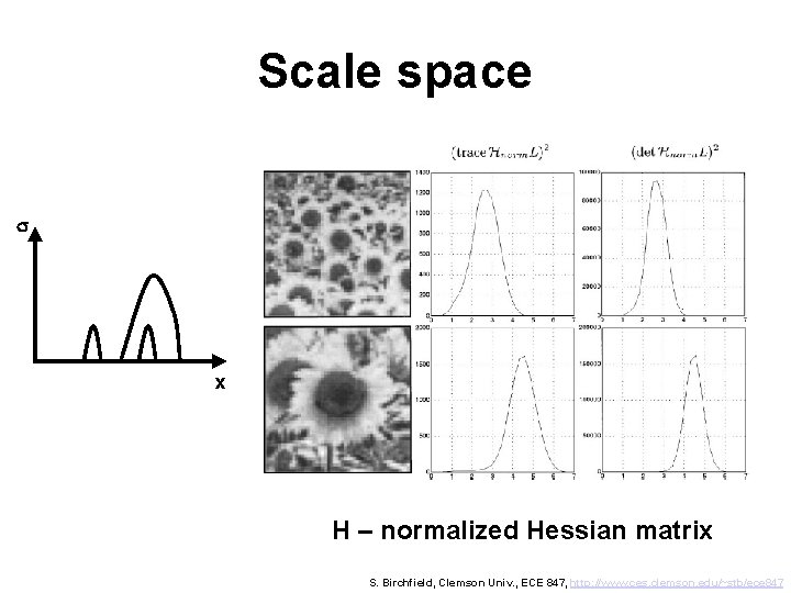
Scale space s x H – normalized Hessian matrix S. Birchfield, Clemson Univ. , ECE 847, http: //www. ces. clemson. edu/~stb/ece 847

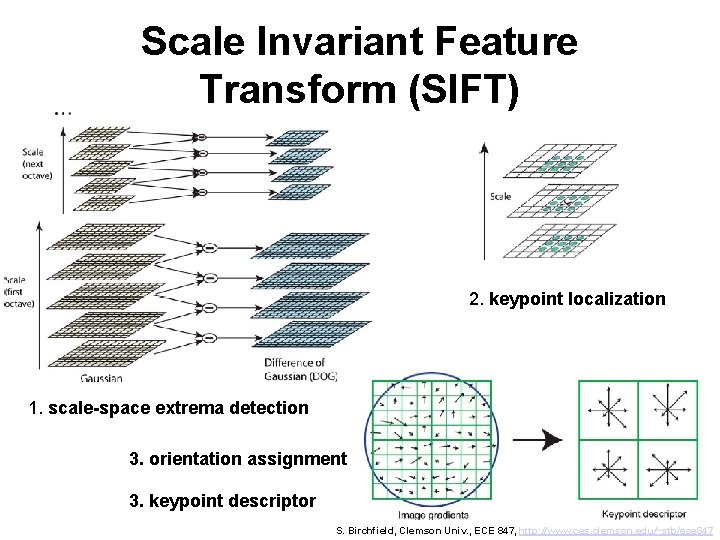
Scale Invariant Feature Transform (SIFT) 2. keypoint localization 1. scale-space extrema detection 3. orientation assignment 3. keypoint descriptor S. Birchfield, Clemson Univ. , ECE 847, http: //www. ces. clemson. edu/~stb/ece 847

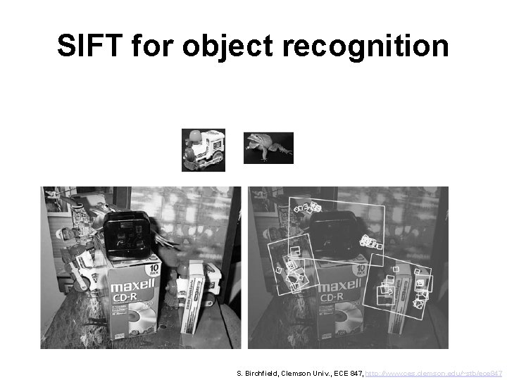
SIFT for object recognition S. Birchfield, Clemson Univ. , ECE 847, http: //www. ces. clemson. edu/~stb/ece 847

Extra slides

Creating 3 x 1 kernels • Sample Gaussian: [a b a] • Normalize by 2 a+b • Value of a and b are determined by s • Examples: (1/4) * [1 2 1] (1/16) * [3 10 3] S. Birchfield, Clemson Univ. , ECE 847, http: //www. ces. clemson. edu/~stb/ece 847

Creating 3 x 1 kernels • Sample Gaussian derivative: [a 0 -a] • Convolution with ramp should yield slope of ramp: [a 0 –a]. * [m+2 m+1 m+0] = 1 a = ½, where m is arbitrary • So normalize by a/2 to get (1/2) * [1 0 -1] • This is the only 3 x 1 Gauss deriv kernel! S. Birchfield, Clemson Univ. , ECE 847, http: //www. ces. clemson. edu/~stb/ece 847

Creating 3 x 1 kernels • Sample Gaussian 2 nd derivative: [a -b a] • Convolution with constant should yield zero: 2 ab=0 b = 2 a: [a -2 a a] • Convolution with changing ramp should yield change in slope: [a -2 a a]. * [p n m] = (p-n) – (n-m) a = 1 • Alternatively, convolution with parabola y=x 2 should yield 2: [a -2 a a]. * [1 0 1] = 2 a = 1 • Either way, this yields: [1 -2 1] • This is the only 3 x 1 Gauss 2 nd deriv kernel! S. Birchfield, Clemson Univ. , ECE 847, http: //www. ces. clemson. edu/~stb/ece 847

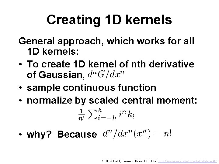
Creating 1 D kernels General approach, which works for all 1 D kernels: • To create 1 D kernel of nth derivative of Gaussian, • sample continuous function • normalize by scaled central moment: • why? Because S. Birchfield, Clemson Univ. , ECE 847, http: //www. ces. clemson. edu/~stb/ece 847