ECE 472572 Digital Image Processing Lecture 5 Image

ECE 472/572 - Digital Image Processing Lecture 5 - Image Enhancement Frequency Domain Filters 09/13/11

Roadmap ¬ Introduction – – Image format (vector vs. bitmap) IP vs. CV vs. CG HLIP vs. LLIP Image acquisition ¬ Image enhancement – – Enhancement vs. restoration Spatial domain methods • – ¬ Perception – • • rods vs. conss (Scotopic vision vs. photopic vision) Fovea and blind spot Flexible lens (near-sighted vs. farsighted) – – • Weber ratio Dynamic range – Image resolution • Sampling vs. quantization – Log trans. vs. Power-law • Gamma correction • Dynamic range compression Contrast stretching vs. HE • What is HE? • Derivation of tran. func. Gray-level vs. Bit plane slicing Image averaging (principle) Mask-based (neighborhood-based) methods spatial filter – – – Brightness adaptation and Discrimination • • – – Structure of human eye • – Point-based methods Smoothing vs. Sharpening filter Linear vs. Non-linear filter Smoothing • Average vs. weighted average • Average vs. Median Sharpening • UM vs. High boosting • 1 st vs. 2 nd derivatives Frequency domain methods 2

Questions ¬ In-depth understanding – Why do we need to conduct image processing in the frequency domain? – What does Fourier series do? – What does the Fourier spectrum of an image tell you? – How to calculate the fundamental frequency? – Why is padding necessary? ¬ Properties – – – Is FT a linear or nonlinear process? What would the FT of a rotated image look like? When implementing FFT, what kind of properties are used? What does the autocorrelation of an image tell you? What is F(0, 0)? Or Why is the center of the FT extremely bright? 3

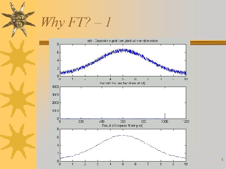
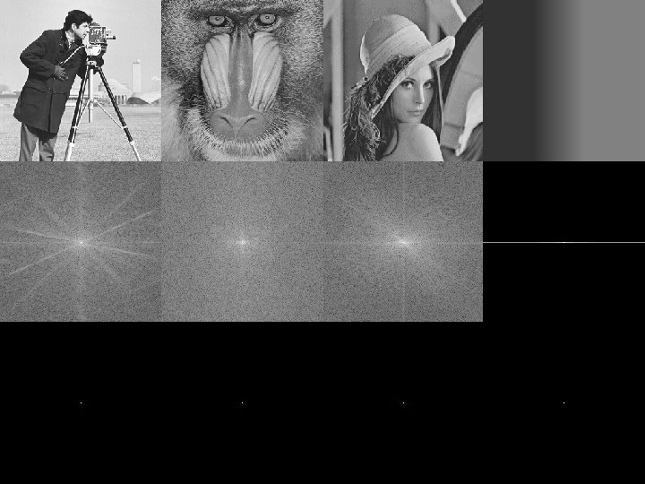
Why FT? – 1 4

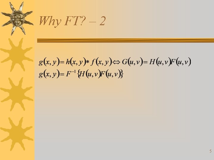
Why FT? – 2 5

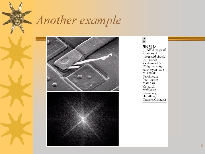
Another example 6

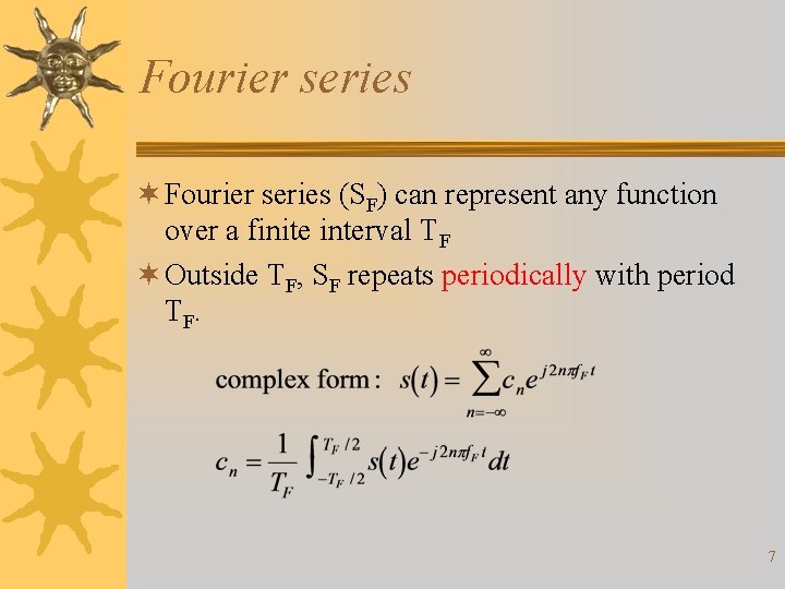
Fourier series ¬ Fourier series (SF) can represent any function over a finite interval TF ¬ Outside TF, SF repeats periodically with period T F. 7

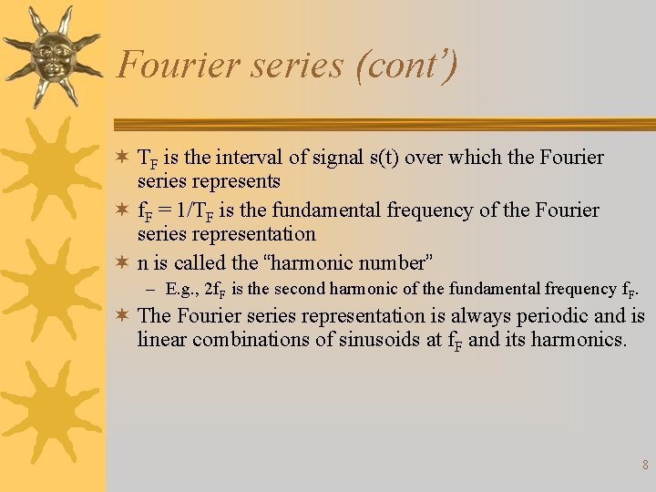
Fourier series (cont’) ¬ TF is the interval of signal s(t) over which the Fourier series represents ¬ f. F = 1/TF is the fundamental frequency of the Fourier series representation ¬ n is called the “harmonic number” – E. g. , 2 f. F is the second harmonic of the fundamental frequency f. F. ¬ The Fourier series representation is always periodic and is linear combinations of sinusoids at f. F and its harmonics. 8

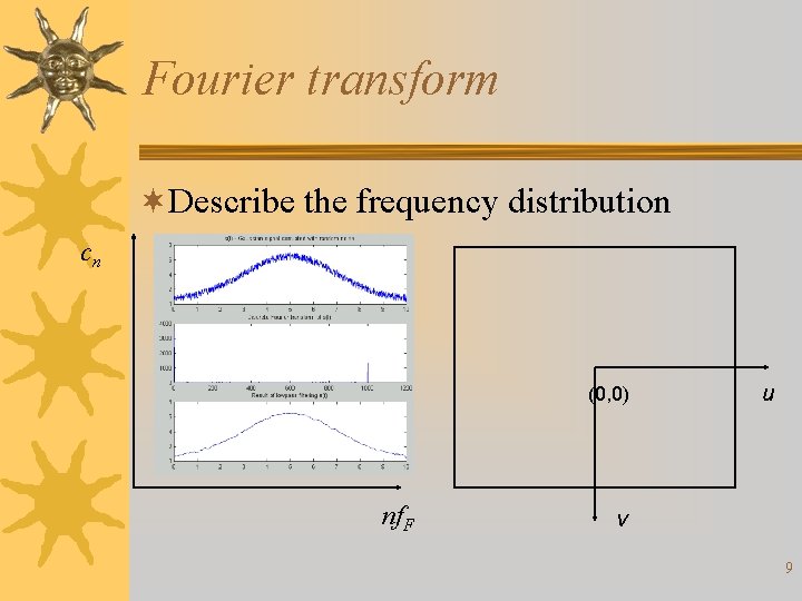
Fourier transform ¬Describe the frequency distribution cn (0, 0) nf. F u v 9

10

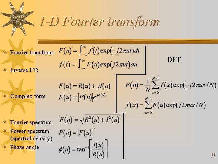
1 -D Fourier transform ¬ Fourier transform: DFT ¬ Inverse FT: ¬ Complex form ¬ Fourier spectrum ¬ Power spectrum (spectral density) ¬ Phase angle 11

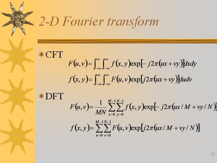
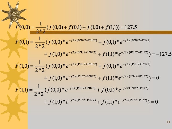
2 -D Fourier transform ¬CFT ¬DFT 12

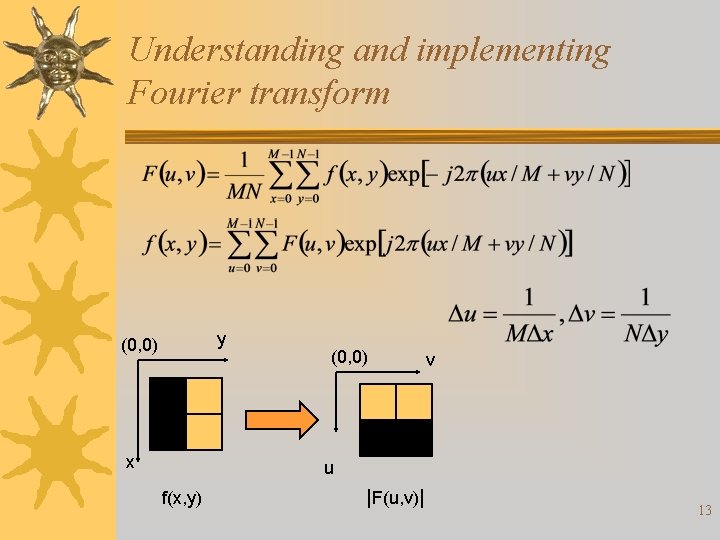
Understanding and implementing Fourier transform y (0, 0) x (0, 0) v u f(x, y) |F(u, v)| 13

14

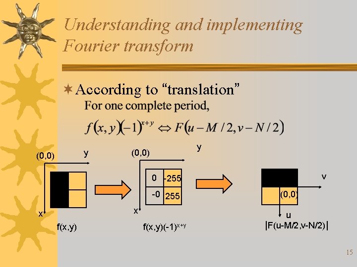
Understanding and implementing Fourier transform ¬According to “translation” y (0, 0) v 0 -255 -0 255 x x f(x, y)(-1)x+y (0, 0) u |F(u-M/2, v-N/2)| 15

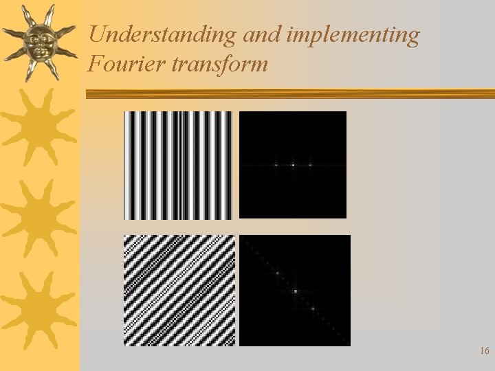
Understanding and implementing Fourier transform 16

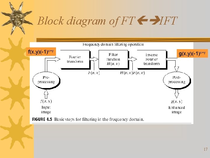
Block diagram of FT IFT f(x, y)(-1)x+y g(x, y)(-1)x+y 17

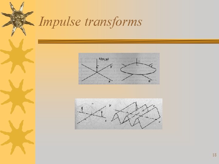
Impulse transforms 18

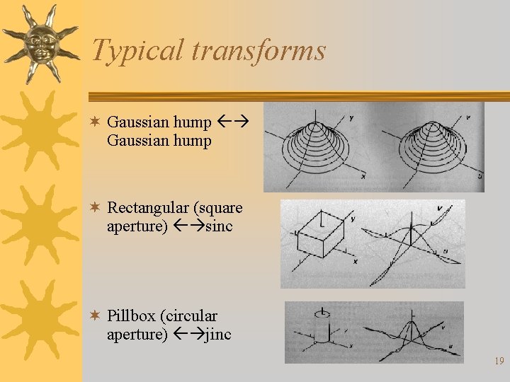
Typical transforms ¬ Gaussian hump ¬ Rectangular (square aperture) sinc ¬ Pillbox (circular aperture) jinc 19

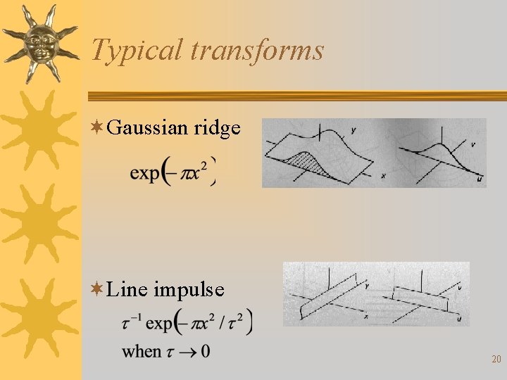
Typical transforms ¬Gaussian ridge ¬Line impulse 20

Reference ¬All figures scanned from R. N. Bracewell’s “Two-Dimensional Imaging, ” Prentice Hall, 1995. 21

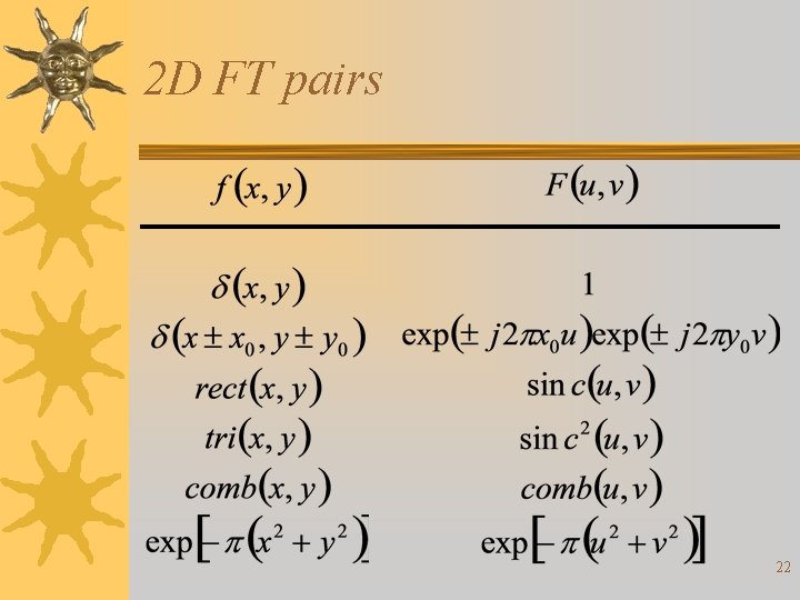
2 D FT pairs 22

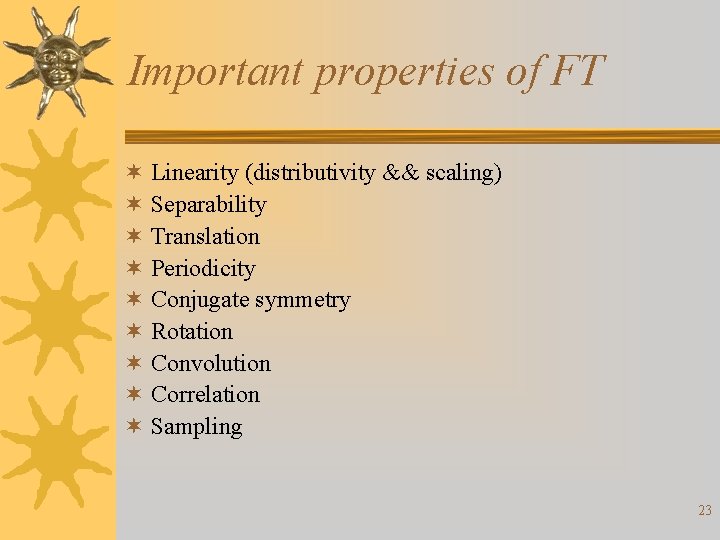
Important properties of FT ¬ Linearity (distributivity && scaling) ¬ Separability ¬ Translation ¬ Periodicity ¬ Conjugate symmetry ¬ Rotation ¬ Convolution ¬ Correlation ¬ Sampling 23

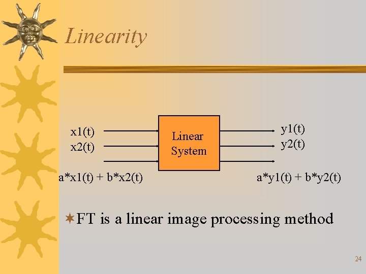
Linearity x 1(t) x 2(t) a*x 1(t) + b*x 2(t) Linear System y 1(t) y 2(t) a*y 1(t) + b*y 2(t) ¬FT is a linear image processing method 24

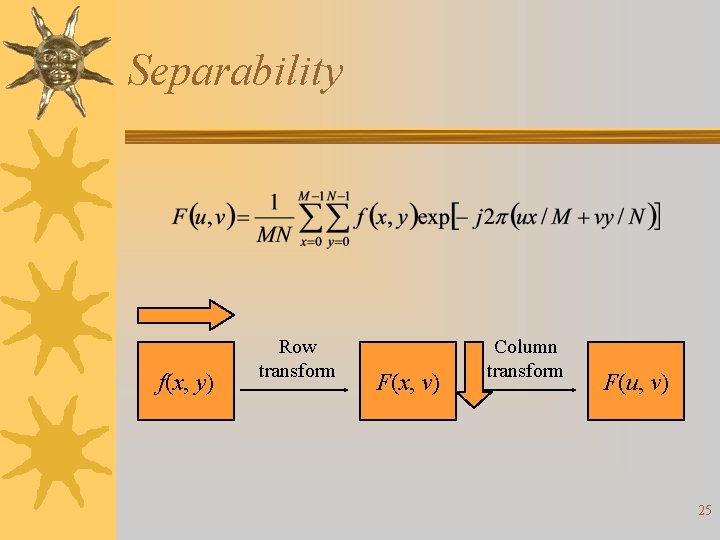
Separability f(x, y) Row transform F(x, v) Column transform F(u, v) 25

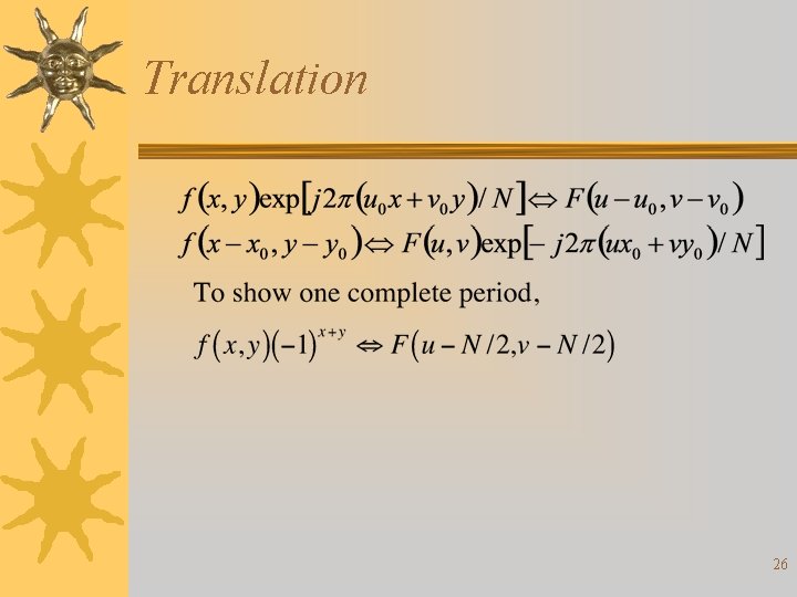
Translation 26

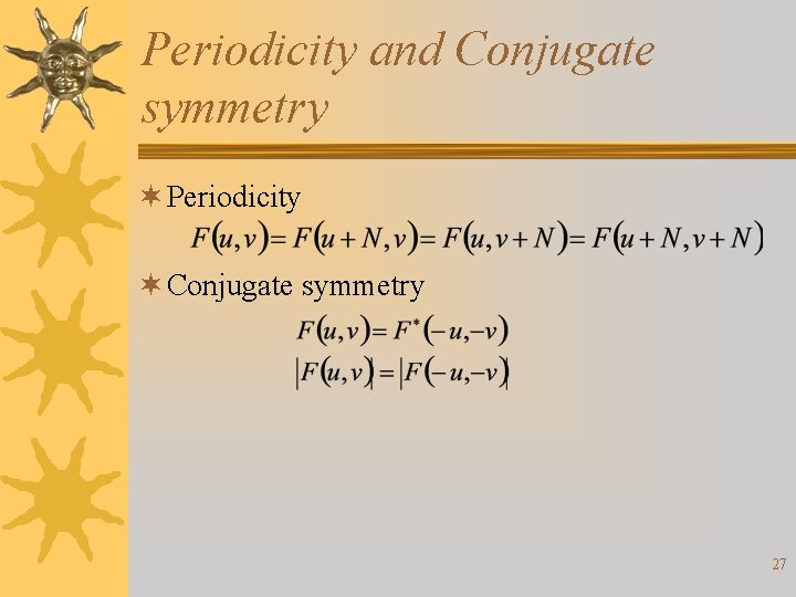
Periodicity and Conjugate symmetry ¬ Periodicity ¬ Conjugate symmetry 27

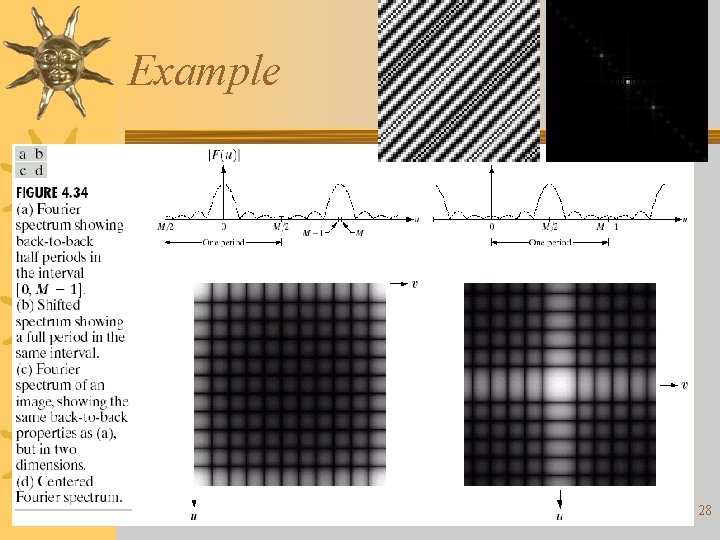
Example 28

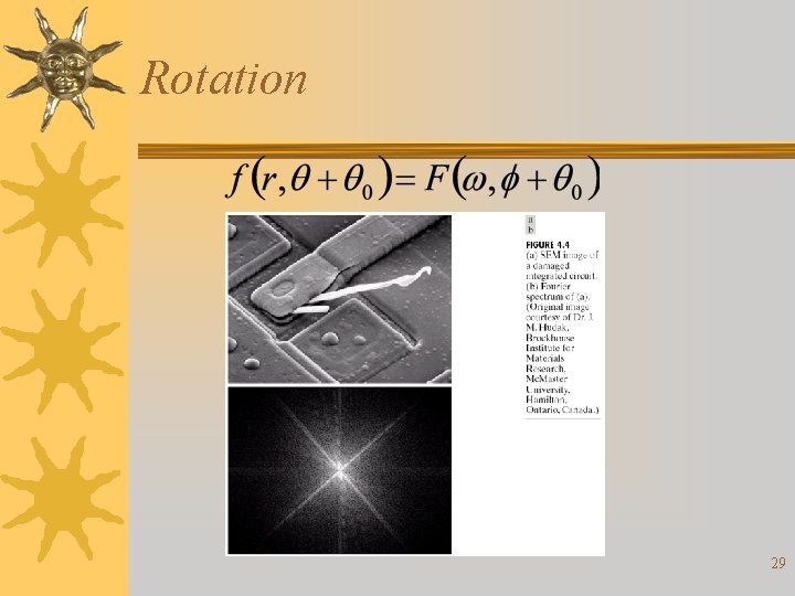
Rotation 29

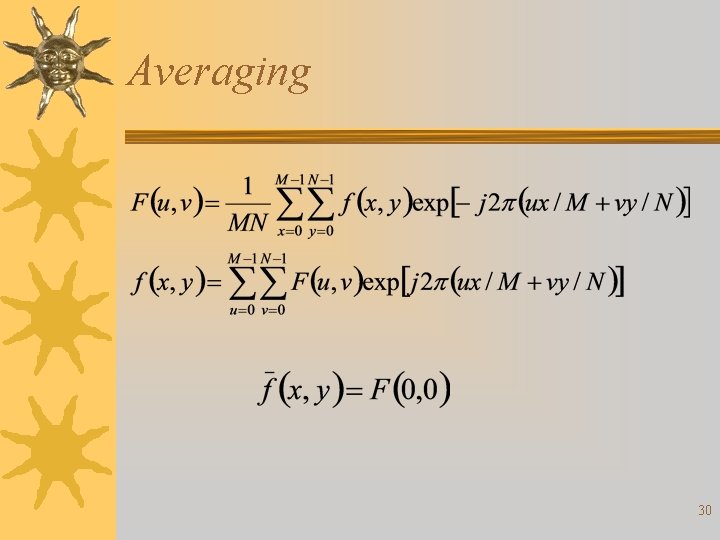
Averaging 30

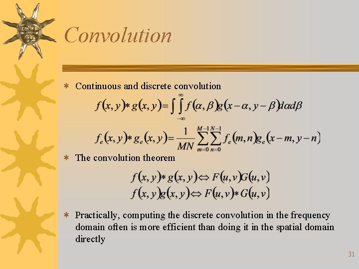
Convolution ¬ Continuous and discrete convolution ¬ The convolution theorem ¬ Practically, computing the discrete convolution in the frequency domain often is more efficient than doing it in the spatial domain directly 31

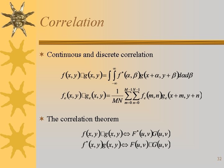
Correlation ¬ Continuous and discrete correlation ¬ The correlation theorem 32

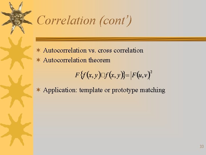
Correlation (cont’) ¬ Autocorrelation vs. cross correlation ¬ Autocorrelation theorem ¬ Application: template or prototype matching 33

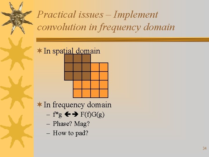
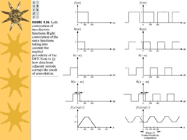
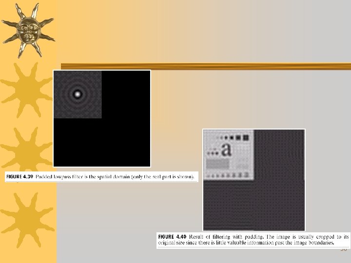
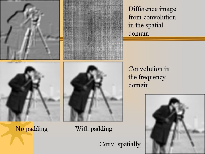
Practical issues – Implement convolution in frequency domain ¬ In spatial domain ¬ In frequency domain – f*g F(f)G(g) – Phase? Mag? – How to pad? 34

35

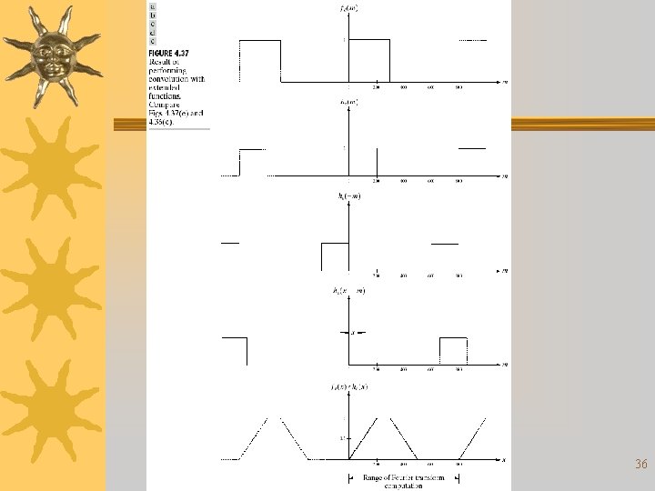
36

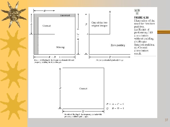
37

38

Difference image from convolution in the spatial domain Convolution in the frequency domain No padding With padding Conv. spatially 39

Different enhancement approaches ¬Lowpass filter ¬Highpass filter ¬Homomorphic filter 40

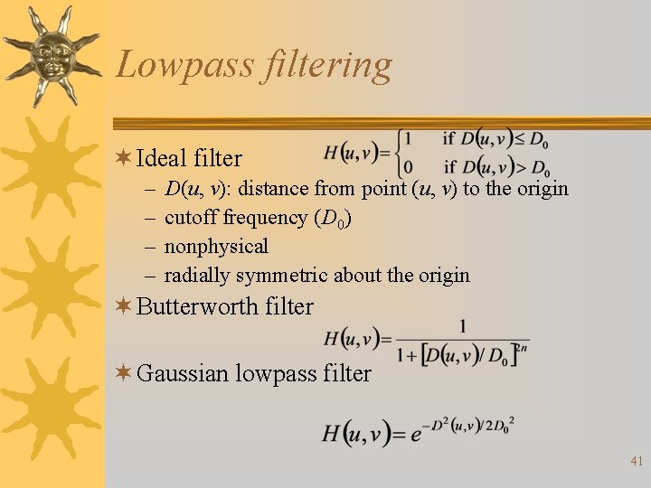
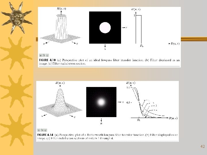
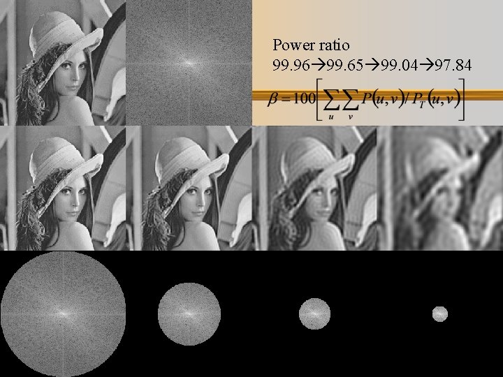
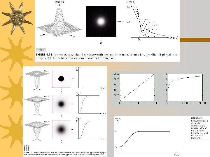
Lowpass filtering ¬ Ideal filter – – D(u, v): distance from point (u, v) to the origin cutoff frequency (D 0) nonphysical radially symmetric about the origin ¬ Butterworth filter ¬ Gaussian lowpass filter 41

42

Power ratio 99. 96 99. 65 99. 04 97. 84 43

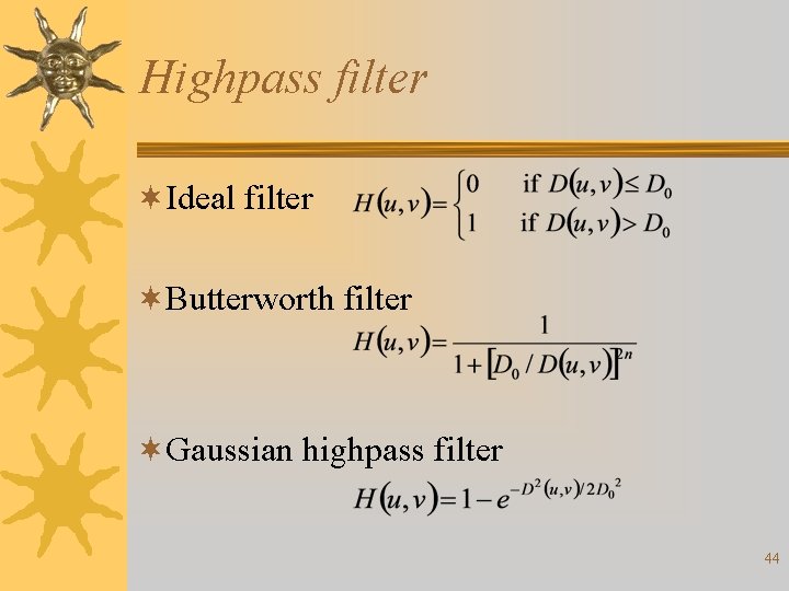
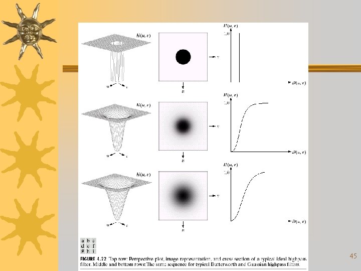
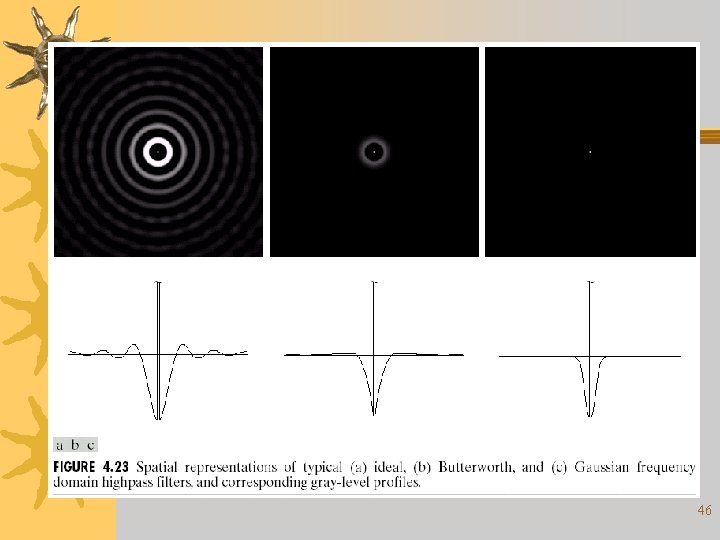
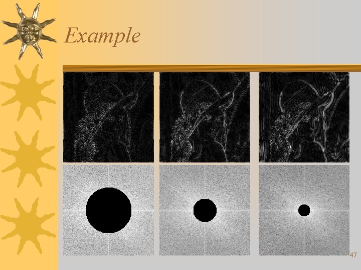
Highpass filter ¬Ideal filter ¬Butterworth filter ¬Gaussian highpass filter 44

45

46

Example 47

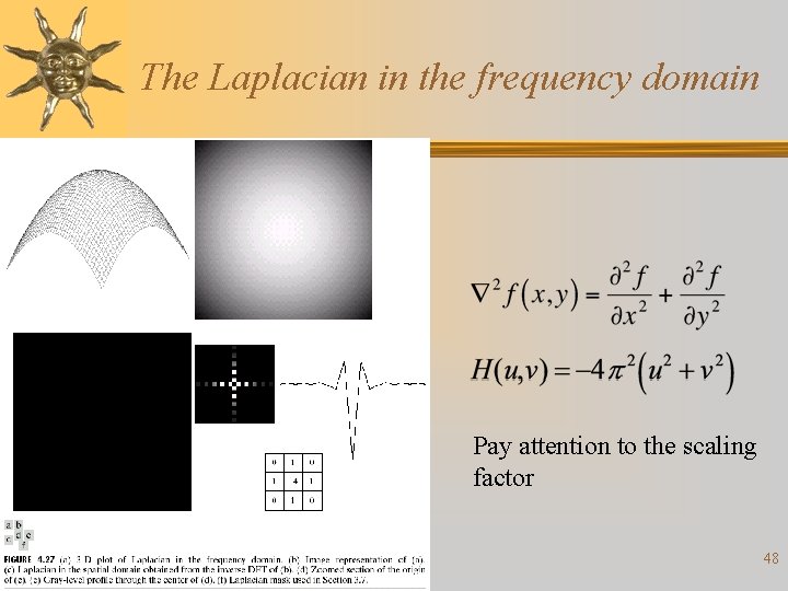
The Laplacian in the frequency domain Pay attention to the scaling factor 48

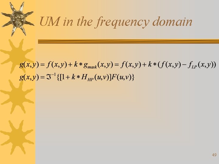
UM in the frequency domain 49

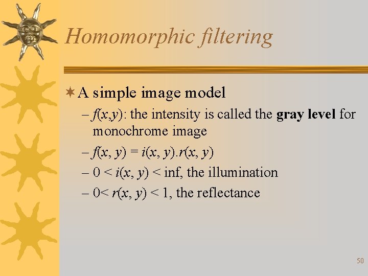
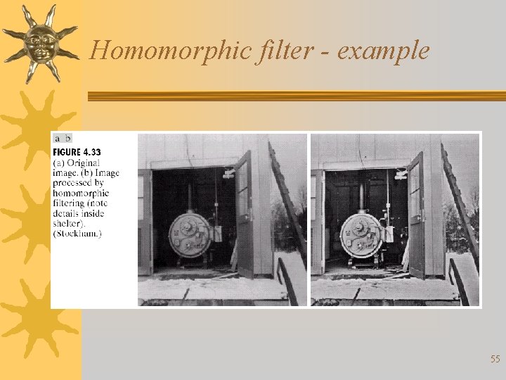
Homomorphic filtering ¬A simple image model – f(x, y): the intensity is called the gray level for monochrome image – f(x, y) = i(x, y). r(x, y) – 0 < i(x, y) < inf, the illumination – 0< r(x, y) < 1, the reflectance 50

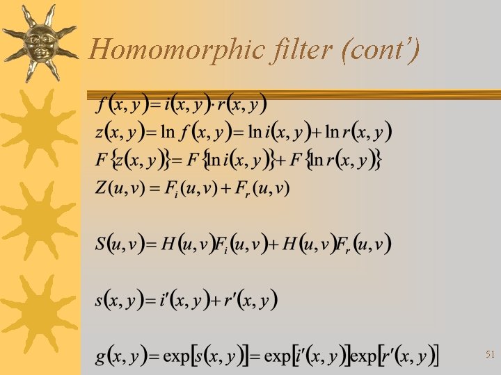
Homomorphic filter (cont’) 51

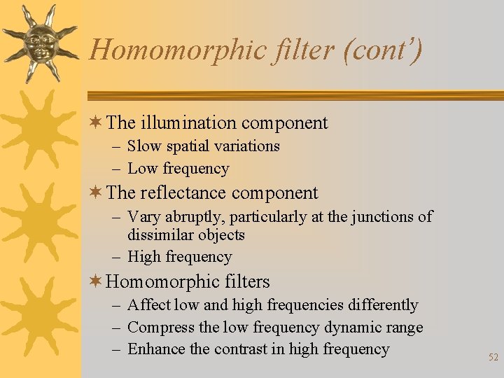
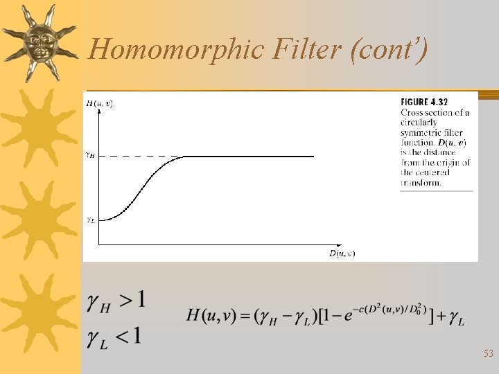
Homomorphic filter (cont’) ¬ The illumination component – Slow spatial variations – Low frequency ¬ The reflectance component – Vary abruptly, particularly at the junctions of dissimilar objects – High frequency ¬ Homomorphic filters – Affect low and high frequencies differently – Compress the low frequency dynamic range – Enhance the contrast in high frequency 52

Homomorphic Filter (cont’) 53

54

Homomorphic filter - example 55

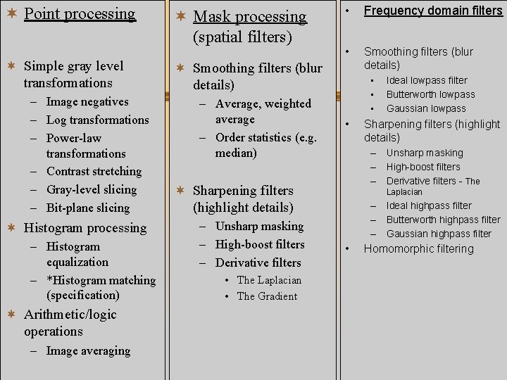
¬ Point processing ¬ Simple gray level transformations – Image negatives – Log transformations – Power-law transformations – Contrast stretching – Gray-level slicing – Bit-plane slicing ¬ Histogram processing – Histogram equalization – *Histogram matching (specification) ¬ Mask processing (spatial filters) • Frequency domain filters • Smoothing filters (blur details) ¬ Smoothing filters (blur details) – Average, weighted average – Order statistics (e. g. median) • • Sharpening filters (highlight details) – Unsharp masking – High-boost filters – Derivative filters - The ¬ Sharpening filters (highlight details) – Unsharp masking – High-boost filters – Derivative filters Ideal lowpass filter Butterworth lowpass Gaussian lowpass Laplacian – Ideal highpass filter – Butterworth highpass filter – Gaussian highpass filter • Homomorphic filtering • The Laplacian • The Gradient ¬ Arithmetic/logic operations – Image averaging 56

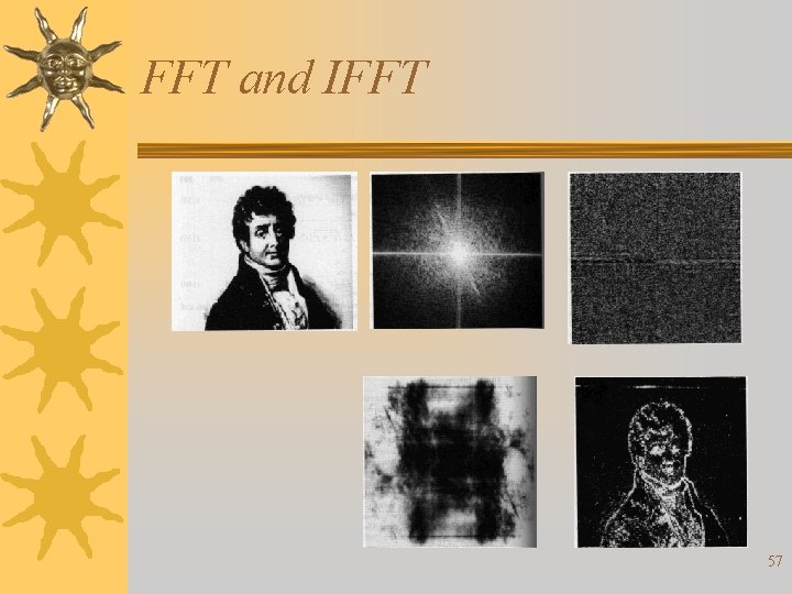
FFT and IFFT 57