Shape and Boundaries ECE 847 Digital Image Processing

Shape and Boundaries ECE 847: Digital Image Processing Stan Birchfield Clemson University

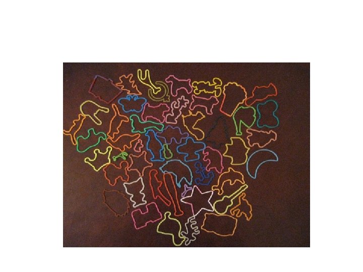
Can you recognize these shapes?

Sometimes edge detectors find the boundary pretty well.

Sometimes it’s not enough.
 • User (or higher-level process) initializes contour • Snake deforms and")
Active contours (Snakes) • User (or higher-level process) initializes contour • Snake deforms and shrink-wraps around object boundary (Diagram courtesy “Snakes, shapes, gradient vector flow”, Xu, Prince)
 • Snake is a parameterized curve: s=0 open curve s=1 s=0")
Active contours (Snakes) • Snake is a parameterized curve: s=0 open curve s=1 s=0 closed curve • Snake is a type of deformable contour
 to image data • Approach: minimize energy functional")
Snakes • Goal: Match curve (boundary) to image data • Approach: minimize energy functional • Like many vision problems, this is underconstrained regularization (impose smoothness prior) image data internal user-supplied (smoothness) Snakes are a top-down approach to segmentation

Internal energy elasticity • 1 st-order term • membrane • a controls tension along spline • stretching balloon or elastic band stiffness • 2 nd-order term • thin plate • b controls rigidity of spline • bending thin plate or bending wire a and b may vary along curve but are usually constant
 and Stiffness (b) Dv v v+Dv • Elasticity draws points together shrinks")
Elasticity (a) and Stiffness (b) Dv v v+Dv • Elasticity draws points together shrinks contour • Stiffness minimizes curvature
 and Stiffness (b) elasticity • Ideal curve is point (circle with zero")
Elasticity (a) and Stiffness (b) elasticity • Ideal curve is point (circle with zero radius) stiffness • Ideal curve is circle (no shrinking)
 Alternatives for")
Image energy We will use only edges (wline = wterm = 0) Alternatives for edge are Key: function must be monotonic non-increasing

Discrete formulation • Curve represented as n points: • Energy: indices are modulo n for closed curve to handle wraparound Note: We will represent the curve simply as a polygon, with the points being the vertices

How to minimize energy • Two approaches: – Finite element and calculus of variations [Kass, Witkin, and Terzopoulos, IJCV 1988] – Dynamic programming [Amini, Weymouth, and Jain, PAMI 1990] • We will only describe the latter, which is much simpler

Basic framework • Start with initial contour • Allow each point to move to one of 9 positions (3 x 3 neighborhood) • Algorithm:

Dynamic programming for snakes • Exploit Markov property of internal energy: point is conditionally independent of all other points, given its immediate neighbors • Dynamic programming can exhaustively consider all 9 n possibilities with just O(92 n) computations
 – Open curve •")
DP Algorithm • Simplifications: – Consider just first-order term (b=0) – Open curve • Construct table (n columns, 9 rows) • Cell (i, j) represents location i for point j • Each cell contains two values: – ij – Cost of best path that ends in point j being in location i – pij – Index of location (0, . . , 8) for previous point j-1 corresponding to this path • Fill table one column at a time from left to right • Minimum ij in last column indicates best curve
 • Each cell must consider all 9 possibilities")
DP st (1 order, open curve) • Each cell must consider all 9 possibilities from previous column • First column ignores internal energy: v 0 v 1 v 2 vi-1 vi Vn-1 (-1, -1) (-1, 0) (-1, 1) j (0, -1) (0, 0) (0, 1) (1, -1) (1, 0) (1, 1) i

Closed curves • Previous algorithm implements • For closed curves, add term to last column for P(vn-1|v 0): • Optimality is lost no matter what m is chosen (could traverse path backwards to find m, but no better than assuming fixed m) In fact, snake will go haywire near v 0 and vn-1 Solutions: • • – Run DP 9 times, using different choice of location for v 0 each time; select the choice with the minimum cost (optimal, but expensive) – Fold curve back onto itself, so that v 1 and vn-1 are both considered in the second column, etc. (optimal, but even more expensive: O(9 4 n) instead of O(92 n)) – Keep adding columns to table until path stabilizes (sounds good, but untested) – Recommended solution: Run DP twice (“probably optimal” in practice, but not guaranteed)

Running DP twice • Solution: – Run once • Pick v 0, run DP (with an extra term in the last column) • Find min cell of last column, trace p back to find path • Discard everything except the location for the point halfway from endpoints, vn/2 – Run again • Set vn/2 to be the new v 0, shifting all other indices down accordingly • Run DP again (with an extra term in the last column) • Find min cell of last column, trace p back to find “probably optimal” path – Now adjust points on snake according to path; this is one iteration • Rationale: The errors due to the open curve assumption should have little effect on points far from the endpoints

Including second-order term • DP will not let us look at future columns: |vi-1 -2 vi+vi+1|2 • So reformulate: |vi-2 vi-1+vi-2|2 • But DP will not let us skip columns, either • So need to increase the state space • Now we have 9 x 9=81 rows and n columns

Including second-order term • Each cell represents locations for two adjacent points • Each cell has 81 elements in previous column, but only 9 are consistent with the cell | (vi-2, vi-1) | (vi-1, vi) | must refer to the same location • Computation is O(93 n) k and j are consistent
 • Simple example: Each point can only move vertically (-1, 0, 1)")
DP (second-order) • Simple example: Each point can only move vertically (-1, 0, 1) only 3 previous cells are consistent v 0 (v 0, v 1) (vi-2, vi-1) (vi-1, vi) Vn-1 (-1), (0) (-1), (1) j (0), (-1) (0), (1), (-1) (1), (0) (1), (1) i

Application: Medical imaging Active Contours and their applications – Julien Jomier - Comp 258 Fall 2002

Examples Hands People Active Contours and their applications – Julien Jomier - Comp 258 Fall 2002

More examples Highway Heart Active Contours and their applications – Julien Jomier - Comp 258 Fall 2002

Drawbacks of snakes • • Sensitive to initial position Sensitive to parameters Small capture range Fails to detect concavities
 • The GVF field is defined to be a vector")
Gradient vector flow (GVF) • The GVF field is defined to be a vector field V(x, y) = • Force equation of GVF snake • V(x, y) is defined such that it minimizes the energy functional f(x, y) is the edge map of the image. C. Xu and J. L. Prince , "Snakes, Shape, and Gradient Vector Flow“, IEEE Transactions on Image Processing, 1998. [from Amyn Poonawala]
 v(x, y) Note")
A look into the vector field components of GVF u(x, y) v(x, y) Note forces also act inside the object boundary!! [from Amyn Poonawala]
![GVF Results Traditional snake GVF snake [from Amyn Poonawala]](http://slidetodoc.com/presentation_image_h2/7b4d0a3461c73d5015ddf0c01dfcf624/image-30.jpg "GVF Results Traditional snake GVF snake [from Amyn Poonawala]")
GVF Results Traditional snake GVF snake [from Amyn Poonawala]

With GVF, the contour can also be initialized across the boundary of object!! Something not possible with traditional snakes. [from Amyn Poonawala]

Level sets • Embed curve in one higher dimension; curve is given by zero level set of implicit function (i. e. , intersection of function with z=0) • Due to J. Sethian and S. Osher 1988 www. math. berkeley. edu/~sethian/level_set. html • Fixes several problems of snakes: – Snake intersects itself – Topology changes

Moving contour using level set • Define level set function z = ( (x, y, t)=0) • Move the level set function, (x, y, t), so that it rises, falls, expands, etc. • By convention, <0 inside the curve and >0 outside the curve from http: //pages. cs. wisc. edu/~fan/Level. Set/Level_presentation/levelsets. ppt

Level set evolution As the surface changes, so does the zero level set from http: //pages. cs. wisc. edu/~fan/Level. Set/Level_presentation/levelsets. ppt

Curve evolution • 2 D: – Curve – Implicit function • Over time: – Curve – Implicit function • Evolution – of curve – of implicit function Simplest implementation:

Advantages of level sets over snakes: • Curve may change topology and form sharp corners (“weak solutions”) • Discrete grid and finite differences approximate solution • Instrinsic geometric properties are easily determined – normal vector – curvature • Formulation is same for 2 D or 3 D

Narrow Band Method

Fast Marching Method • J. Sethian, 1996 • Special case that assumes the velocity field, F, never changes sign. That is, contour is either always expanding or always shrinking • Can convert problem to a stationary formulation on a discrete grid where the contour is guaranteed to cross each grid point at most once from http: //pages. cs. wisc. edu/~fan/Level. Set/Level_presentation/levelsets. ppt
 = time at which the contour crosses")
Fast Marching Method • Compute T(x, y) = time at which the contour crosses grid point (x, y) • At any height, T, the surface gives the set of points reached at time T from http: //pages. cs. wisc. edu/~fan/Level. Set/Level_presentation/levelsets. ppt
 (iii) (iv) from http: //pages. cs. wisc. edu/~fan/Level. Set/Level_presentation/levelsets. ppt")
Fast Marching Method (i) (iii) (iv) from http: //pages. cs. wisc. edu/~fan/Level. Set/Level_presentation/levelsets. ppt
 incrementally: 1. Build")
Fast Marching Algorithm • Construct the arrival time surface T(x, y) incrementally: 1. Build the initial contour 2. Incrementally add on to the existing surface the part that corresponds to the contour moving with speed F • Builds level set surface by scaffolding the surface patches farther and farther away from the initial contour from http: //pages. cs. wisc. edu/~fan/Level. Set/Level_presentation/levelsets. ppt

Fast Marching Visualization from http: //pages. cs. wisc. edu/~fan/Level. Set/Level_presentation/levelsets. ppt

Mumford-Shah • Mumford-Shah functional captures how well reconstructed function matches original image • Regularization term enforces smoothness, but not at boundaries contour reconstruction image domain D. Mumford and J. Shah. Boundary detection by minimizing functionals. CVPR, 1985.

Chan-Vese model • Snakes and level sets have several problems: – Small basin of attraction (edges) – initial contour must surround object (or be completely contained within it • Chan-Vese (2001) propose – segmenting image using model of interior and exterior – level set function is used to represent the curve (or equivalently the binary mask of the interior region) – for simplicity, assume interior and exterior both have approximately constant intensity (but different from each other)
 • Goal is to minimize energy functional where • and –")
Chan-Vese (cont. ) • Goal is to minimize energy functional where • and – – m, n, li, and lo are constants G is contour w is interior region bounded by G ci and co are average intensities inside and outside G
 • Heaviside function: • regularized Heaviside function: vs. (other functions are")
Chan-Vese (cont. ) • Heaviside function: • regularized Heaviside function: vs. (other functions are possible) • derivative: Dirac delta function “hard threshold, not differentiable” “soft threshold, differentiable”
 • H(f(x, y)) is approximately 1 inside contour, and approximately 0")
Chan-Vese (cont. ) • H(f(x, y)) is approximately 1 inside contour, and approximately 0 outside • Therefore,
 • Now express the gradient of H(f(x, y)) in terms of")
Chan-Vese (cont. ) • Now express the gradient of H(f(x, y)) in terms of the gradient of f(x, y): • Therefore,
 • Because we are minimizing an energy functional, you shouldn’t be")
Chan-Vese (cont. ) • Because we are minimizing an energy functional, you shouldn’t be surprised that we will be using the Euler-Lagrange equation • In preparation, note that • where
 • Now let us take some derivatives: • And,")
Chan-Vese (cont. ) • Now let us take some derivatives: • And,
 • Now we plug these into the Euler-Lagrange equation: • where")
Chan-Vese (cont. ) • Now we plug these into the Euler-Lagrange equation: • where the divergence operator of a vector field is defined as
 • Substituting yields our result: • If we could solve this")
Chan-Vese (cont. ) • Substituting yields our result: • If we could solve this equation for , we would be done • But nobody knows how to do this • Instead we treat the LHS as a deviation from the true solution, and apply gradient descent iterations of the form assuming
 • As the implicit function f evolves, it can generate kinks")
Chan-Vese (cont. ) • As the implicit function f evolves, it can generate kinks • To alleviate this problem, it is common to periodically re-initialize f to the signed distance to the contour • This is done by computing y(x), the distance to the zero level set (e. g. , using chamfering). Then set

Chan-Vese algorithm fx / | f| fx | f| f fy div( f / | f| ) fy / | f|
 image Df f (k+1)")
Chan-Vese algorithm | f| div( f / | f| ) image Df f (k+1) f (k) reinitialized f (k+1)

Determining intensities • Algorithm description assumes ci and co are known • To find them, differentiate E: average gray level in region average gray level outside region

Complete algorithm • Initialize G and • Use to compute ci and co • Iterate – – – Compute div( / | | ), | | Compute D Set (k+1) = (k) + D Compute G from Reinitialize Use to compute ci and co Until convergence
 vs. | | -- we use latter, Chan. Vese use")
Implementation issues • h() vs. | | -- we use latter, Chan. Vese use former • atan vs. 1/(1+e^-z) Heaviside -- we use latter, Chan-Vese use former • divergence based on finite differences (one step) vs. derivative of Gaussian -- we use latter, Chan. Vese use former
 1 2 3 4 5 6 7 8")
Chan-Vese results iteration 99 0 (convergence) 1 2 3 4 5 6 7 8 9 10 11 12

Compare with Ridler-Calvard

A related problem We’ll do something easier than finding the whole boundary. Finding the best path between two boundary points. [from snakes. ppt]

How do we decide how good a path is? Which of two paths is better?

Discrete Grid • Contour should be near edge. • Strength of gradient. • Contour should be smooth (good continuation). • Low curvature • Low change of direction of gradient.
, p(2), … p(n). Where • d(p(j),")
Combine into a cost function • Path: p(1), p(2), … p(n). Where • d(p(j), p(j+1)) is distance between consecutive grid points (ie, 1 or sqrt(2). • g(p(j)) measures strength of gradient • l is some parameter • f measures smoothness, curvature.
 and")
One example cost function f is the angle between the gradient at p(j-1) and p(j). Or it could more directly measure curvature of the curve. (Loosely based on “Dynamic Programming for Detecting, Tracking, and Matching Deformable Contours”, by Geiger, Gupta, Costa, and Vlontzos, IEEE Trans. PAMI 17(3)294 -302, 1995. )

So How do we find the best Path? A Curve is a path through the grid. Cost depends on each step of the path. We want to minimize cost.

Map problem to Graph Weight represents cost of going from one pixel to another. Next term in sum.

Dijkstra’s shortest path algorithm 4 9 5 1 0 3 3 3 2 • link cost Algorithm 1. init node costs to , set p = seed point, cost(p) = 0 2. expand p as follows: for each of p’s neighbors q that are not expanded – set cost(q) = min( cost(p) + cpq, cost(q) ) (Seitz)

Dijkstra’s shortest path algorithm • Algorithm 4 9 5 1 0 3 3 2 3 1. init node costs to , set p = seed point, cost(p) = 0 2. expand p as follows: for each of p’s neighbors q that are not expanded – set cost(q) = min( cost(p) + cpq, cost(q) ) » if q’s cost changed, make q point back to p – put q on the ACTIVE list (if not already there)

Dijkstra’s shortest path algorithm 4 9 3 2 5 4 9 5 2 1 1 0 3 3 4 3 3 2 3 • Algorithm 3 2 5 3 3 1. init node costs to , set p = seed point, cost(p) = 0 2. expand p as follows: for each of p’s neighbors q that are not expanded – set cost(q) = min( cost(p) + cpq, cost(q) ) » if q’s cost changed, make q point back to p – put q on the ACTIVE list (if not already there) 3. set r = node with minimum cost on the ACTIVE list 4. repeat Step 2 for p = r

Dijkstra’s shortest path algorithm 4 3 • Algorithm 4 3 6 3 2 5 4 9 5 2 1 1 0 3 3 4 3 3 2 5 3 3 1. init node costs to , set p = seed point, cost(p) = 0 2. expand p as follows: for each of p’s neighbors q that are not expanded – set cost(q) = min( cost(p) + cpq, cost(q) ) » if q’s cost changed, make q point back to p – put q on the ACTIVE list (if not already there) 3. set r = node with minimum cost on the ACTIVE list 4. repeat Step 2 for p = r

Application: Intelligent Scissors
 demo")
Results (Seitz Class) demo

Lessons • Perceptual grouping, middle-level knowledge needed for boundary detection • Fully automatic solutions not good enough yet

B-splines • Splines are elastic beams used by draftsmen for designing curves in ships • Splines assume shape that minimizes the strain energy • B-splines are mathematical representation of curves in the 2 D plane • Related to Bezier curves

Continuity • C 0 means the curve points vary smoothly – Curve is a set of connected points – Two joined segments share endpoints • C 1 means the 1 st derivative is continuous (and C 0) – Two joined segments share tangents where they meet • C 2 means the 2 nd derivative is continuous (and C 0 and C 1) – Two joined segments share curvature where they meet

Uniform cubic B-splines • Simplest is the uniform cubic B-spline • Curve is • Represented by control points • Example: 9 control points, 6 segments from www. cs. uwec. edu/~stevende/cs 455/handouts/Modeling. ppt

Blending functions • Uniform B-spline: All blending functions are the same from www. cs. uwec. edu/~stevende/cs 455/handouts/Modeling. ppt

Using B-splines • Let • Then where needed to maintain C 2 continuity

Computing slope of B-spline • Take partial derivatives: • Slope:

Constructing B-spline • Given data points • Suppose we wish to interpolate • If ubar is an integer, • All together:
 • Need to add two more equations: • Yielding: •")
Constructing B-spline (cont. ) • Need to add two more equations: • Yielding: • This is invertible. Given Pi, solve for Qi
 example shapes point model scatter plot")
Active shape models • Point distribution model (PDM) example shapes point model scatter plot T. F. Cootes and C. J. Taylor and D. H. Cooper and J. Graham. "Active shape models - their training and application". Computer Vision and Image Understanding, (61): 38— 59, 1995.
 Run PCA to capture the shape variations Effects of")
Active shape models (cont. ) Run PCA to capture the shape variations Effects of varying the first three eigenvectors:

Generalized cylinders • We have already seen skeletons

Shape context Example: Handwritten characters are different using pixel-wise comparison, but shape is similar: How to capture this notion? Shape context: • simple, intuitive descriptor • easy to compute • robust to occlusions, deformations S. Belongie, J. Malik, and J. Puzicha. "Shape Matching and Object Recognition Using Shape Contexts". IEEE Transactions on Pattern Analysis and Machine Intelligence, 24 (24): 509– 521, April 2002.

Computing shape context • Represent shape as set of boundary points (may be interior or exterior) -- from Canny, for example • Sample subset of points randomly (with uniform spacing, preferably) • For each point, its shape context is a histogram: using a log-polar grid

Example shape contexts

Matching shape contexts Two points are matched using c 2 distance between their shape contexts: Two shapes are matched by summing the matching costs of the points: where the permutation p is found by solving the bipartite matching problem using • the classic Hungarian method, or • the Jonker-Volgenant approach (faster) Note: Outliers are handled by adding dummy nodes with constant cost e

Invariance • Shape contexts are inherently invariant to translation • Scale invariance is achieved by normalizing all radial distances by the mean distance between the n 2 point pairs in the shape • Robustness to small nonlinear transformations, occlusions, and outliers is achieved by the histogram • If desired, rotation invariance can be achieved by using relative reference frames defined by the tangent vector of each point

Modeling transformations Given correspondences, a plane transformation can be found to map the points to one another Thin plate spline (TPS) is a 2 D generalization of cubic splines

Application: Handwriting recognition Errors on the MNIST database

Application: MPEG-7

Application: Trademark retrieval

Shapemes • Uses vector quantization on the shape contexts of know shapes ‘S’. • By k-means clustering, k-shapemes are obtained. So each d-bin hist is replaced by shapeme label. • Hence each ‘s’ shape contexts with d-bin histograms is reduced to single histogram with k bins from Nalin Pradeep

Results from Nalin Pradeep
- Slides: 96