Course 5 Edge Detection Course 5 Edge Detection

Course 5 Edge Detection

Course 5 Edge Detection Image Features: local, meaningful, detectable parts of an image. l edge l corner l texture l … Edges: Edges points, or simply edges, are pixels at or around which the image values undergo a sharp variation.

Usually, edges are classified as： l step edge, l ridge edge l roof edge. We will emphasize on step edge detection in our discussions.

1. Edge detection: 1) Goal: 2) Given an image corrupted by acquisition noise, locate the edges most likely to be generated by scene elements not by noise. 2) Operations required in edge detection i) Noise smoothing: suppress as much of the image noise as possible, without destroying the edges. In the absence of specific information of image, assume the noise white and Gaussian.

ii) Edge Enhancement: Design a filter corresponding to edges; that is, the filter’s output is large at edge pixel and low elsewhere, so edge an be located as the maximum in filter’s output. iii) Edge Location: Decide which local maximum in the filter’s output are edges and which are just caused by noise.

3) Edge descriptions: l l edge normal: the direction (unit vector) of the maximum intensity variation at edge pixels. Edge normal is perpendicular to the edge direction: perpendicular to edge normal, and therefore tangent to the contour. edge position: the pixel position where the edge is located. edge strength: the measurement of local image contrast, e. g. , intensity variation along an edge normal.

2. Gradient Based Edge Detection: 1) Gradient: 2) Magnitude 3) Direction

Note: The direction of edge normal is perpendicular to the edge. In computation, gradient is approximated by: 1 -1 1 GX = G Y = -1 for symmetry, 1 1 GX = G -1 1 Y = -1 -1 -1 1

2) Roberts Operator 3) Sobel Operator: — avoid having the gradient calculated about an interpolated point between pixels.

where c is constant, a 0 a 1 a 2 a 7 [i, j] a 3 a 6 a 5 a 4 e. g. , c = 2 -1 0 1 1 2 1 -2 0 Sx= S y= 0 0 -2 -1 -1 And, 0 1 -1

3. Lap. Lacian Operator ----Second derivative of a smoothed step edge gives a function that crosses zero at the location of the edge. The second derivative of a 2 D function is Laplacian.

In discrete computation: Or, by template, 0 1 -4 1 0

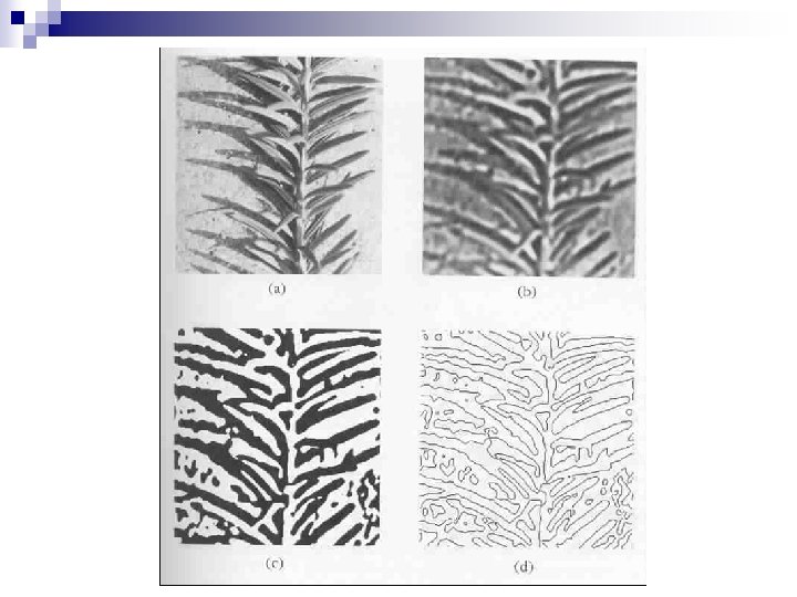
4. Lap. Lacian of Gaussian (LOG) LOG combines Guassian filter with the Lap. Lasian for edge detection: — smoothing filter using a Gaussian — edge enhancement using Laplassian — edge localization by detecting zero-crossing Let g(x, y) be Gaussian filter. f(x, y) be noise corrupted image; h(x, y) be LOG , then:

Then Log is :

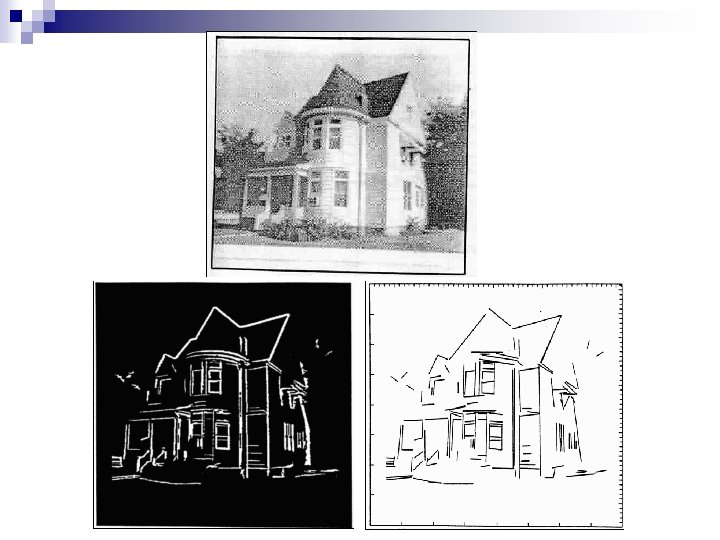
5. Canny Edge Detector: So far, canny operator has been considered as the best of edge detector. Canny operator consists of four basic processes: — smooth image with a Gaussian filter — compute gradient magnitude and orientation using finite difference approximation. -1 1 -1 -1

— Applying nonmaxima suppression to gradient magnitude to identify edge locations. — We double thresholding to detect and link edges. 1) Canny-Enhancer (smoothing and enhancement) 2) a) Apply Gaussian smoothing to input image I, obtaining 3) 4) where G is Gaussian filter.

b) For each pixel [i, j] , compute gradient component Jx and Jy by finite-difference estimate: Edge strength Edge normal c) Form output: Strength image: Es , formed by es[i, j], Orientation image: E 0 , formed by e 0[i, j].

2) Nonmaxima-supperation The input images are Es and E 0 , the edge strength image and edge orientation image. Consider four directions d 1, d 2, d 3, d 4 identified by 00, 450, 900, 1350 orientations. For each pixel [i, j]: a) find direction dk which best approximates the direction of E 0[i, j]. b) Along the direction dk, check the two neighbors of pixel [i, j]. If Es[i, j] is greater than both of its neighbors, set IN[i, j] = Es[i, j]; otherwise, EN[i, j] = 0. The output image IN consists of thinned edge points.

3) Double threshold and edge link Input image IN and E 0 , choose two thresholds Th and TL such that Th >TL a) Locate an unvisited edge point IN[i, j] which satisfies I N[i, j]> Th. b) Follow IN in the directions perpendicular to edge normal as long as IN>Th. Save the satisfied edge points. c) When the tracing process ended there IN<Th, look for connectivity with the condition IN>TL. .

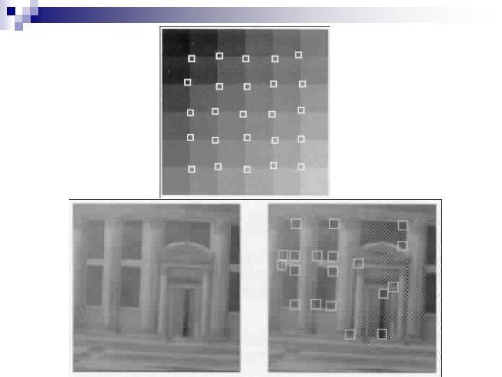
d) When edge gap can be bridged up (where IN > Th. ), go to step b). If it cannot find further connectivity of IN > TL, go to step a). 6. Corner Detection: Corner features have advantages: — more meaningfully defined in scene. — less likely to generate false features. — corners are easier to match than edge points.

For an image I, consider a point p with intensity gradient Ix and Iy. In a neighborhood N of p form the structure matrix C: The key is to find the eigenvalues and corresponding eigenvector of matrix C. — if image is uniform, C = 0. And — if image consists of only an ideal step edge, rank of c is 1, and λ 1 > 0, λ 2 = 0 ,

the direction of eigenvector of corresponds to the edge normal. — if image contains an ideal corner, then The eigenvector of corresponds to the stronger edge of the corner; the eigenvector of to the weaker edge.

Algorithm (Tomasi and Kanade, 1991) Input image is I, two preset parameters: T——threshold on smaller eignvalue N——window size of neighborhood. a) Compute image gradient over I. b) For each image point, from structure matrix C in its neighborhood of window. c) Compute the eigenvalues .

d) If , save point P in list L e) Sort L in decreasing order. f) Scan L from top to bottom. For each point P, delete all its neighborhood that appears in the list L, so that output points do not have overlapped neighborhood.

7. Line Detection (Liu and Huang, 1991) Line features have advantages: — more meaningfully defined in scene — less affected by noise — subpixel accuracy — easier to match(less false matches) Input image: I, preset parameter: T — gradient threshold — parameter of Gaussian filter

Algorithm: a) Use Gaussian filter to smooth image I, output is G. b) Calculate gradient of image G and its magnitude and orientation for each point. c) Thresholding gradient magnitude M by value T to get a binary image S, line support region image. when M[i, j] >T, S[i, j]=1, otherwise S[i, j]=0.

d) Based on the direction of edge normal, segment each connected regions Si into subregion; in each subregion, the orientations do not differ much. e) Suppose the equation of image line is ax + by + c = 0 The distance from a point in the support region to the line is

f) For each subregion obtained in step d), minimize the sum of distance from point to the line. g) Use least-square to solve for parameters a, b and c. Thus, line is found. Note: the choice of threshold value of T is not critical in the algorithm.