CH 5 Image Restoration 5 1 A model

CH 5. Image Restoration 5. 1 A model of the image degradation/ restoration process 5. 2 Noise models 5. 3 Restoration in the presence of noise only-spatial filtering 5. 4 Noise reduction by freq. domain filtering 5. 5 Linear, position-invariant degradation 5. 6 Estimating the degradation function 5. 7 Inverse filtering, Wiener filtering, Constraint least squares filtering, Geometric mean filter 1

Chapter 5 Image Restoration • Image Restoration is distinguished from Image Enhancement (CH. 3 -4) - IE: heuristic, subjective process, e. g. contrast stretching - IR: objective process, e. g. removing blur • The degradation modeling and inverse process to get back to the original image 2

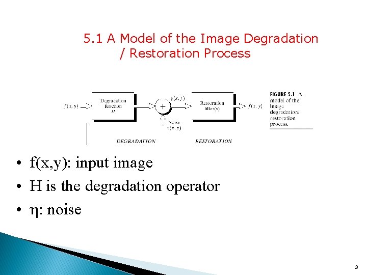
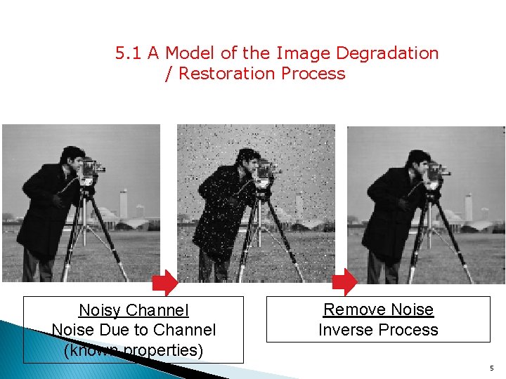
5. 1 A Model of the Image Degradation / Restoration Process • f(x, y): input image • H is the degradation operator • η: noise 3

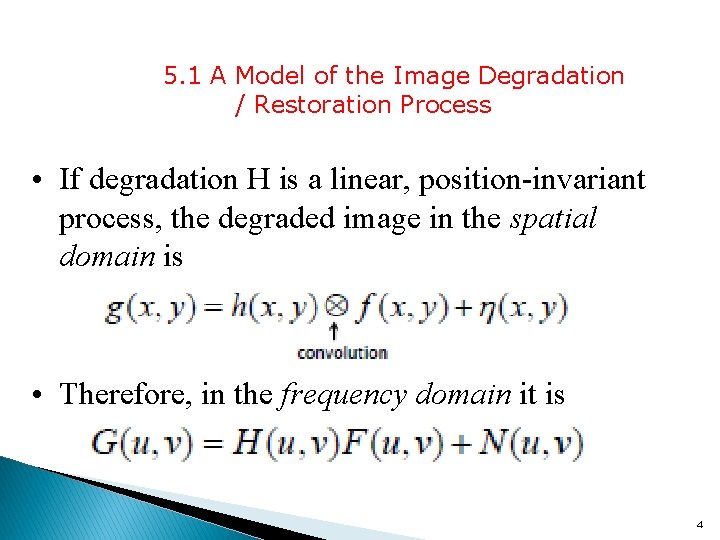
5. 1 A Model of the Image Degradation / Restoration Process • If degradation H is a linear, position-invariant process, the degraded image in the spatial domain is • Therefore, in the frequency domain it is 4

5. 1 A Model of the Image Degradation / Restoration Process Noisy Channel Noise Due to Channel (known properties) Remove Noise Inverse Process 5

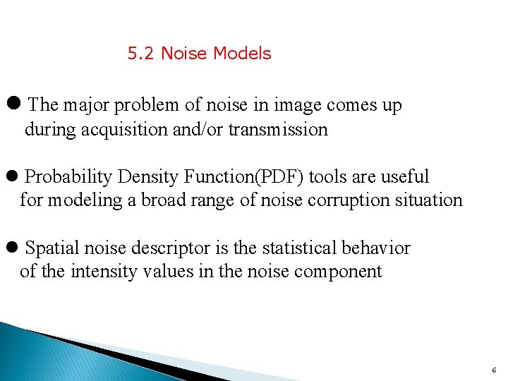
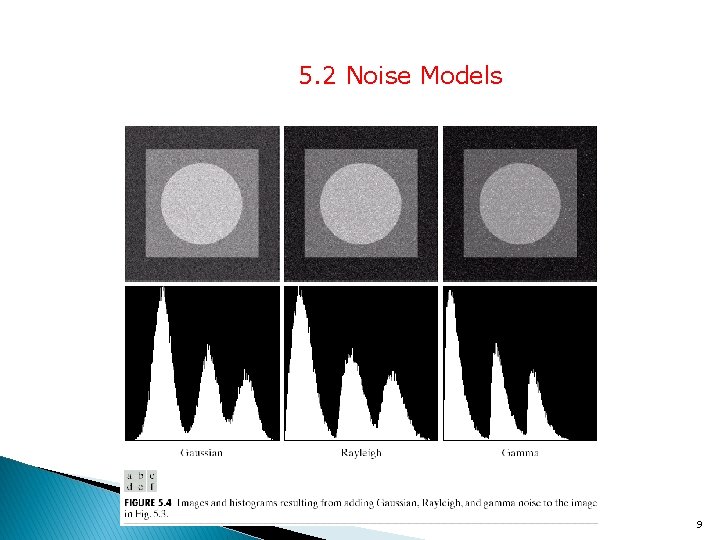
5. 2 Noise Models l The major problem of noise in image comes up during acquisition and/or transmission l Probability Density Function(PDF) tools are useful for modeling a broad range of noise corruption situation l Spatial noise descriptor is the statistical behavior of the intensity values in the noise component 6

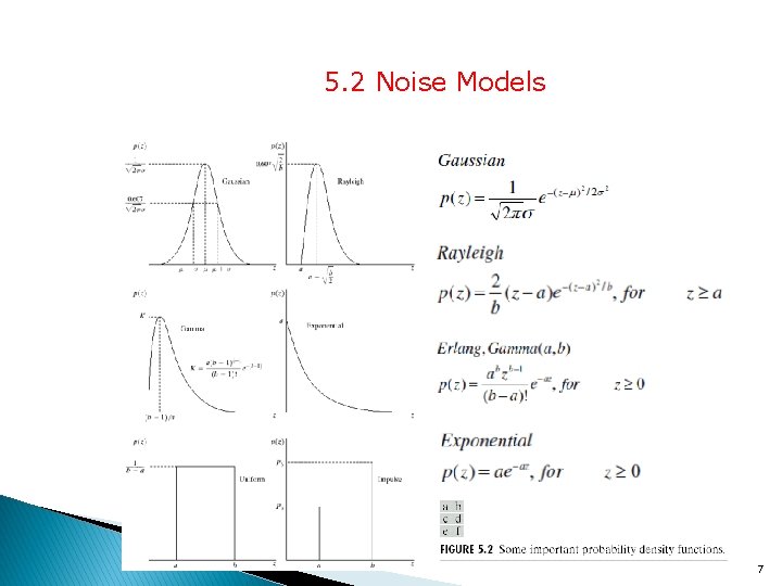
5. 2 Noise Models 7

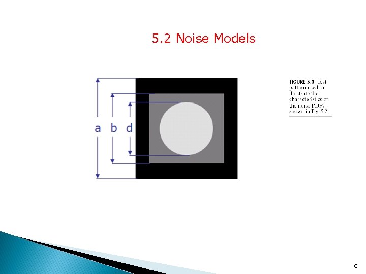
5. 2 Noise Models 8

5. 2 Noise Models 9

5. 2 Noise Models 10

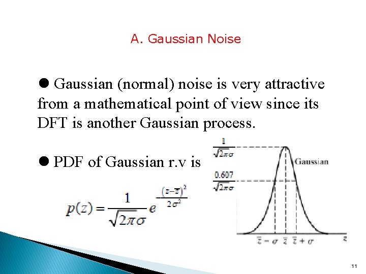
A. Gaussian Noise l Gaussian (normal) noise is very attractive from a mathematical point of view since its DFT is another Gaussian process. l PDF of Gaussian r. v is 11

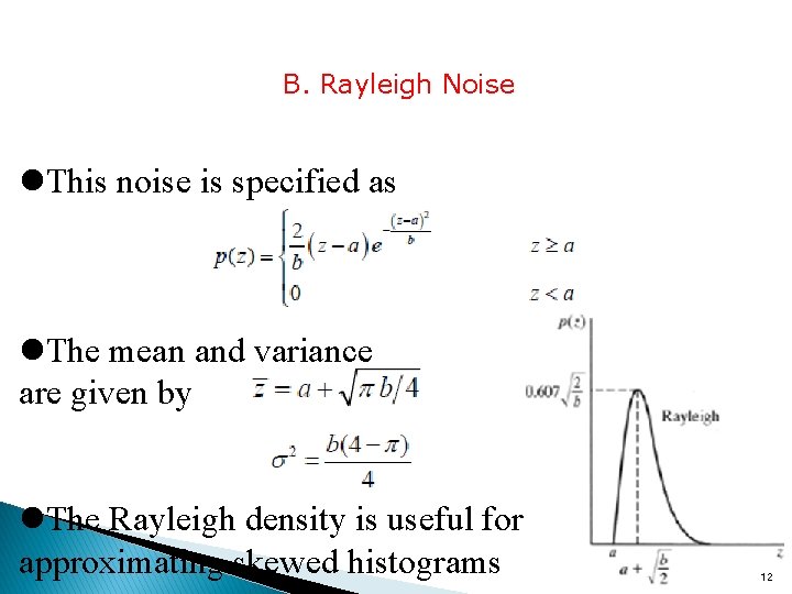
B. Rayleigh Noise l. This noise is specified as l. The mean and variance are given by l. The Rayleigh density is useful for approximating skewed histograms 12

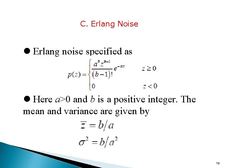
C. Erlang Noise l Erlang noise specified as l Here a>0 and b is a positive integer. The mean and variance are given by 13

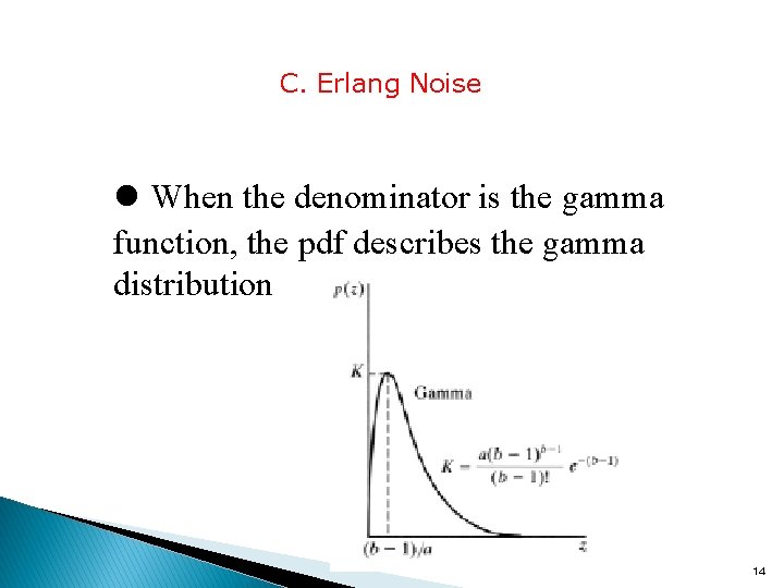
C. Erlang Noise l When the denominator is the gamma function, the pdf describes the gamma distribution 14

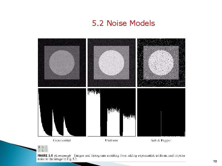
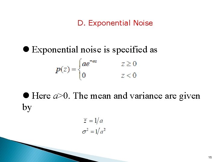
D. Exponential Noise l Exponential noise is specified as l Here a>0. The mean and variance are given by 15

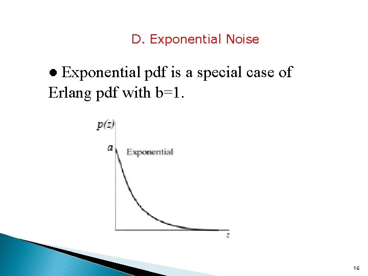
D. Exponential Noise Exponential pdf is a special case of Erlang pdf with b=1. l 16

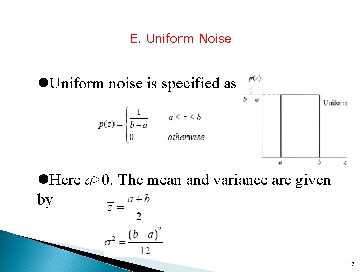
E. Uniform Noise l. Uniform noise is specified as l. Here a>0. The mean and variance are given by 17

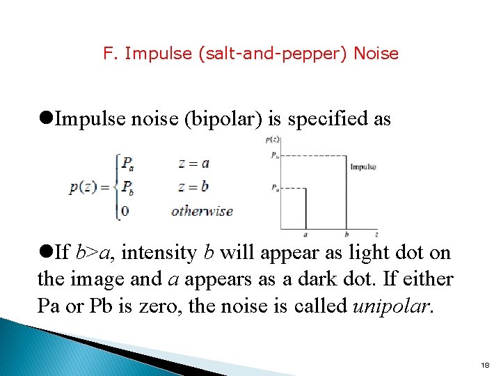
F. Impulse (salt-and-pepper) Noise l. Impulse noise (bipolar) is specified as l. If b>a, intensity b will appear as light dot on the image and a appears as a dark dot. If either Pa or Pb is zero, the noise is called unipolar. 18

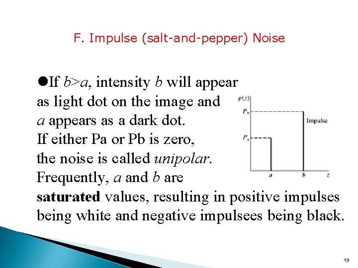
F. Impulse (salt-and-pepper) Noise l. If b>a, intensity b will appear as light dot on the image and a appears as a dark dot. If either Pa or Pb is zero, the noise is called unipolar. Frequently, a and b are saturated values, resulting in positive impulses being white and negative impulsees being black. 19

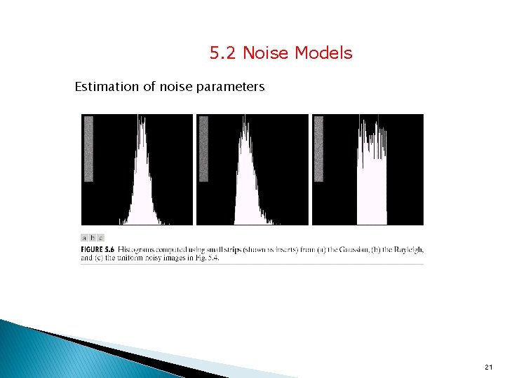
5. 2 Noise Models l It is possible to estimate the parameters of the PDF from small patch of background intensity, when only images are available l The shape of histogram identifies the closest PDF match 20

5. 2 Noise Models Estimation of noise parameters 21

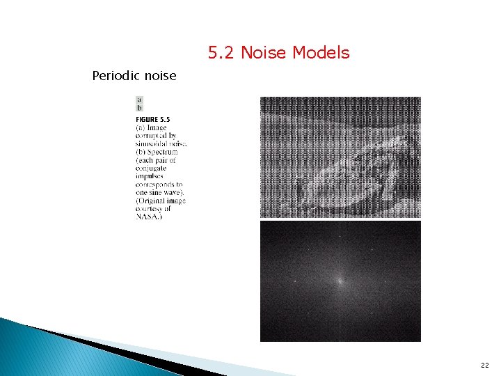
5. 2 Noise Models Periodic noise 22

23

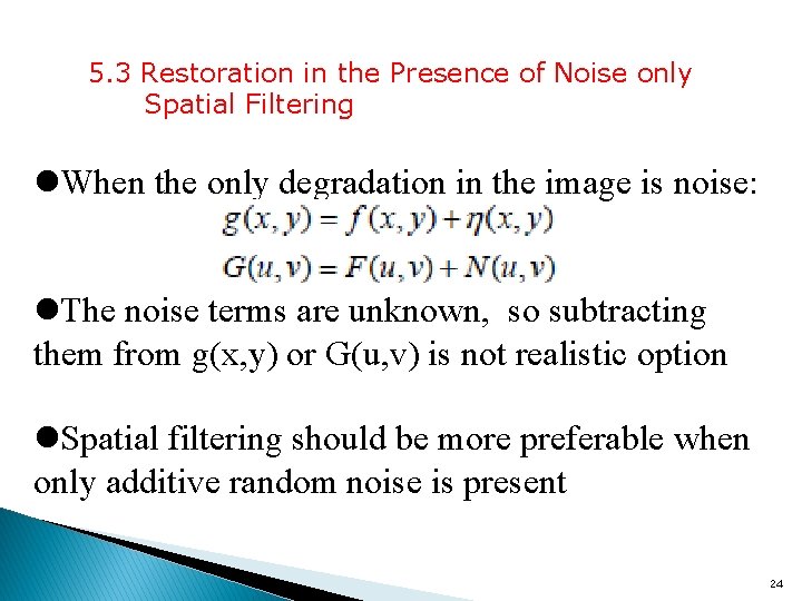
5. 3 Restoration in the Presence of Noise only Spatial Filtering l. When the only degradation in the image is noise: l. The noise terms are unknown, so subtracting them from g(x, y) or G(u, v) is not realistic option l. Spatial filtering should be more preferable when only additive random noise is present 24

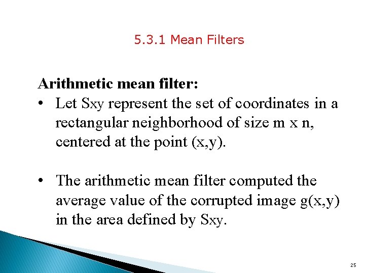
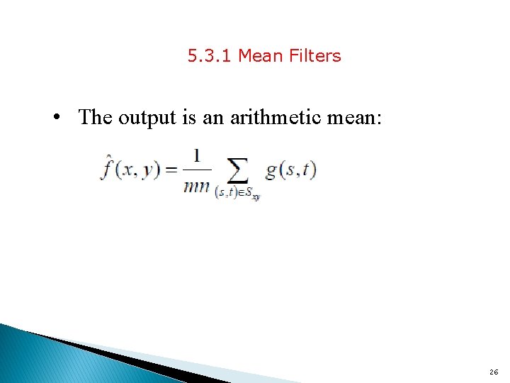
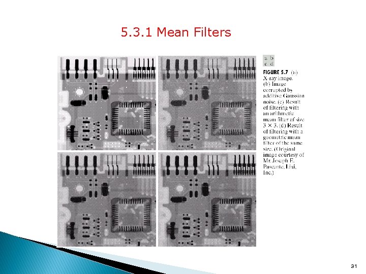
5. 3. 1 Mean Filters Arithmetic mean filter: • Let Sxy represent the set of coordinates in a rectangular neighborhood of size m x n, centered at the point (x, y). • The arithmetic mean filter computed the average value of the corrupted image g(x, y) in the area defined by Sxy. 25

5. 3. 1 Mean Filters • The output is an arithmetic mean: 26

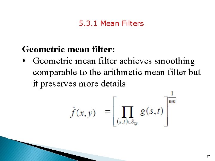
5. 3. 1 Mean Filters Geometric mean filter: • Geometric mean filter achieves smoothing comparable to the arithmetic mean filter but it preserves more details 27

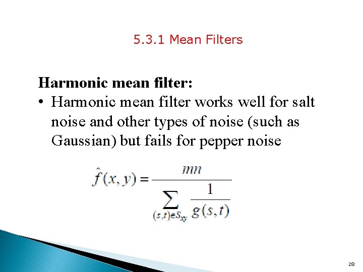
5. 3. 1 Mean Filters Harmonic mean filter: • Harmonic mean filter works well for salt noise and other types of noise (such as Gaussian) but fails for pepper noise 28

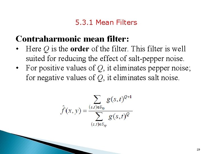
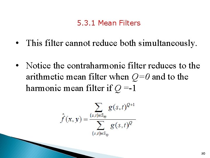
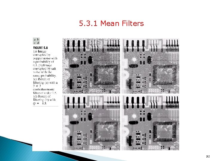
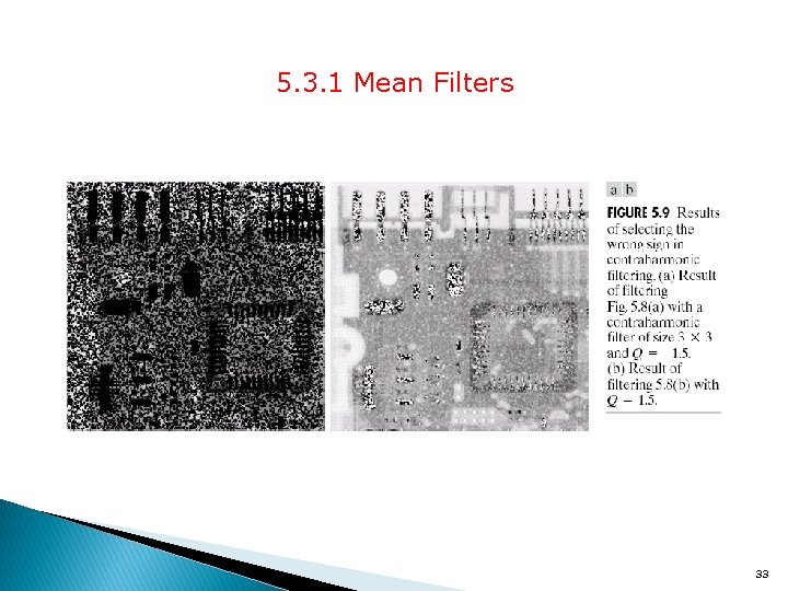
5. 3. 1 Mean Filters Contraharmonic mean filter: • Here Q is the order of the filter. This filter is well suited for reducing the effect of salt-pepper noise. • For positive values of Q, it eliminates pepper noise; for negative values of Q, it eliminates salt noise. 29

5. 3. 1 Mean Filters • This filter cannot reduce both simultaneously. • Notice the contraharmonic filter reduces to the arithmetic mean filter when Q=0 and to the harmonic mean filter if Q =-1 30

5. 3. 1 Mean Filters 31

5. 3. 1 Mean Filters 32

5. 3. 1 Mean Filters 33

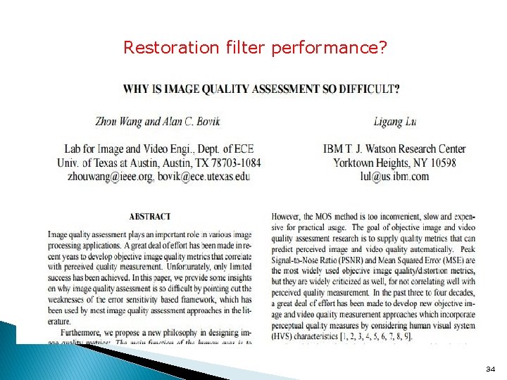
Restoration filter performance? 34

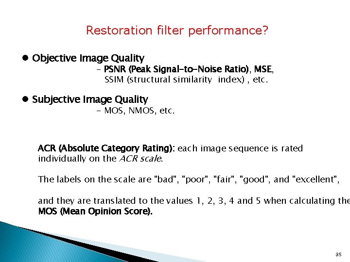
Restoration filter performance? l Objective Image Quality - PSNR (Peak Signal-to-Noise Ratio), MSE, SSIM (structural similarity index) , etc. l Subjective Image Quality - MOS, NMOS, etc. ACR (Absolute Category Rating): each image sequence is rated individually on the ACR scale. The labels on the scale are "bad", "poor", "fair", "good", and "excellent", and they are translated to the values 1, 2, 3, 4 and 5 when calculating the MOS (Mean Opinion Score). 35

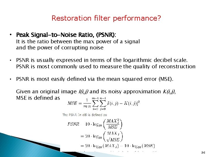
Restoration filter performance? • Peak Signal-to-Noise Ratio, (PSNR): It is the ratio between the max power of a signal and the power of corrupting noise • PSNR is usually expressed in terms of the logarithmic decibel scale. PSNR is most commonly used to measure the quality of reconstruction • PSNR is most easily defined via the mean squared error (MSE). Given an original image I(i, j) and its noisy approximation K(i, j), MSE is defined as: 36

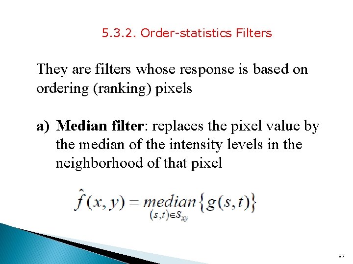
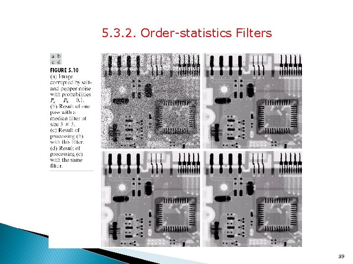
5. 3. 2. Order-statistics Filters They are filters whose response is based on ordering (ranking) pixels a) Median filter: replaces the pixel value by the median of the intensity levels in the neighborhood of that pixel 37

5. 3. 2. Order-statistics Filters • Median filters provide excellent results for certain types of noise with considerably less blurring than linear smoothing filters of the same size • These filters are very effective against both bipolar and unipolar noise contaminations 38

5. 3. 2. Order-statistics Filters 39

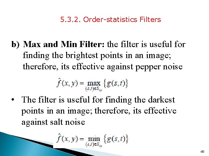
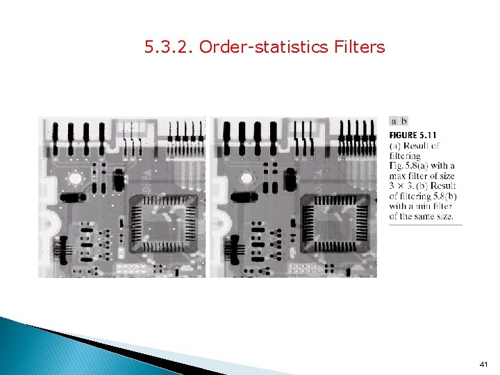
5. 3. 2. Order-statistics Filters b) Max and Min Filter: the filter is useful for finding the brightest points in an image; therefore, its effective against pepper noise • The filter is useful for finding the darkest points in an image; therefore, its effective against salt noise 40

5. 3. 2. Order-statistics Filters 41

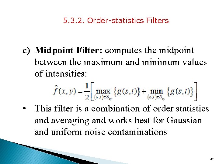
5. 3. 2. Order-statistics Filters c) Midpoint Filter: computes the midpoint between the maximum and minimum values of intensities: • This filter is a combination of order statistics and averaging and works best for Gaussian and uniform noise contaminations 42

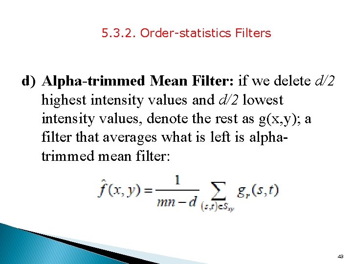
5. 3. 2. Order-statistics Filters d) Alpha-trimmed Mean Filter: if we delete d/2 highest intensity values and d/2 lowest intensity values, denote the rest as g(x, y); a filter that averages what is left is alphatrimmed mean filter: 43

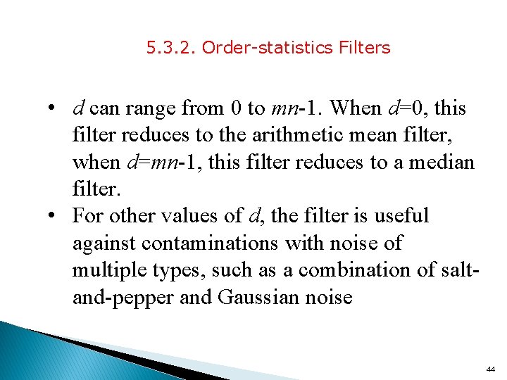
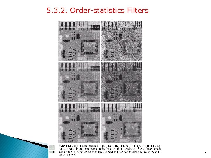
5. 3. 2. Order-statistics Filters • d can range from 0 to mn-1. When d=0, this filter reduces to the arithmetic mean filter, when d=mn-1, this filter reduces to a median filter. • For other values of d, the filter is useful against contaminations with noise of multiple types, such as a combination of saltand-pepper and Gaussian noise 44

5. 3. 2. Order-statistics Filters 45

5. 3. 3 Adaptive Filters • The behavior of adaptive filters changes based on statistical characteristics (var. mean) of the image inside the filter region Sxy, m x n local window region - The mean gives a measure for average intensity in the region - The variance characterizes contrast in that region, they both are reasonable parameters to base an adaptive filter. 46

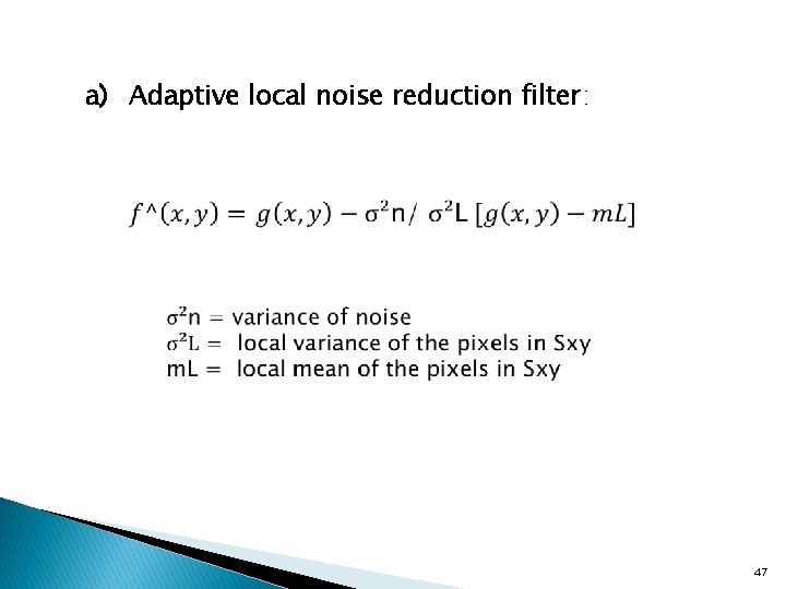
a) Adaptive local noise reduction filter: 47

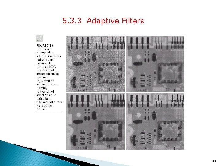
5. 3. 3 Adaptive Filters 48

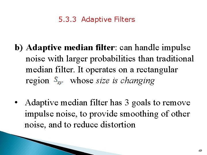
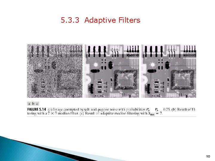
5. 3. 3 Adaptive Filters b) Adaptive median filter: can handle impulse noise with larger probabilities than traditional median filter. It operates on a rectangular region whose size is changing • Adaptive median filter has 3 goals to remove impulse noise, to provide smoothing of other noise, and to reduce distortion 49

5. 3. 3 Adaptive Filters 50

Summary 1. A Model of the Image Degradation/ Restoration Process 2. Noise Models: • Gaussian, Rayleigh, Erlang, Exponential, Uniform, Impulse 3. Restoration in the Presence of Noise Only-Spatial Filtering: • Mean (Arithmethic, Geometric, Harmonic, Contraharmonic mean filter) • Order-statistic (Median, Max. /Min. , Midpoint, Alphatrimmed mean filter) 4. Restoration filter performance – PSNR, MSE, MOS , etc.