Digital Image Processing Lecture 10 Image Restoration March

Digital Image Processing Lecture 10: Image Restoration March 28, 2005 Prof. Charlene Tsai Digital Image Processing Lecture 10

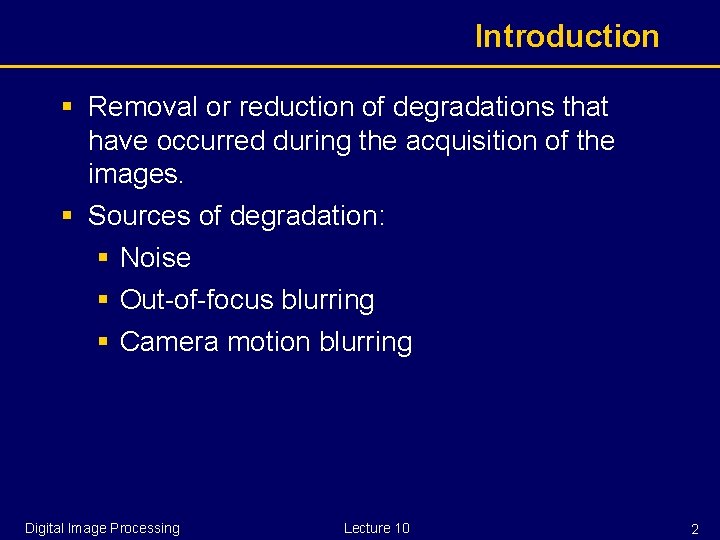
Introduction § Removal or reduction of degradations that have occurred during the acquisition of the images. § Sources of degradation: § Noise § Out-of-focus blurring § Camera motion blurring Digital Image Processing Lecture 10 2

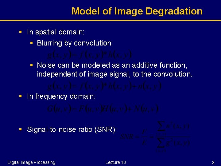
Model of Image Degradation § In spatial domain: § Blurring by convolution: § Noise can be modeled as an additive function, independent of image signal, to the convolution. § In frequency domain: § Signal-to-noise ratio (SNR): Digital Image Processing Lecture 10 3

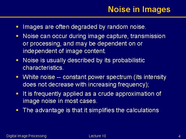
Noise in Images § Images are often degraded by random noise. § Noise can occur during image capture, transmission or processing, and may be dependent on or independent of image content. § Noise is usually described by its probabilistic characteristics. § White noise -- constant power spectrum (its intensity does not decrease with increasing frequency); § It is frequently applied as a crude approximation of image noise in most cases. § The advantage is that it simplifies the calculations Digital Image Processing Lecture 10 4

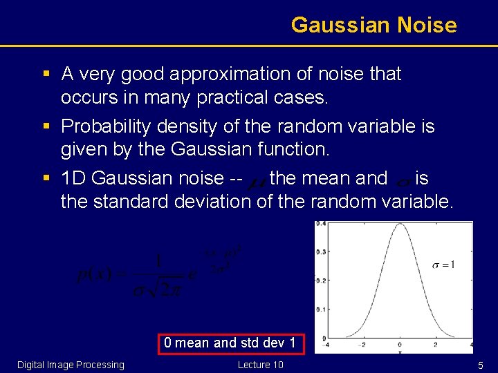
Gaussian Noise § A very good approximation of noise that occurs in many practical cases. § Probability density of the random variable is given by the Gaussian function. § 1 D Gaussian noise -- the mean and is the standard deviation of the random variable. 0 mean and std dev 1 Digital Image Processing Lecture 10 5

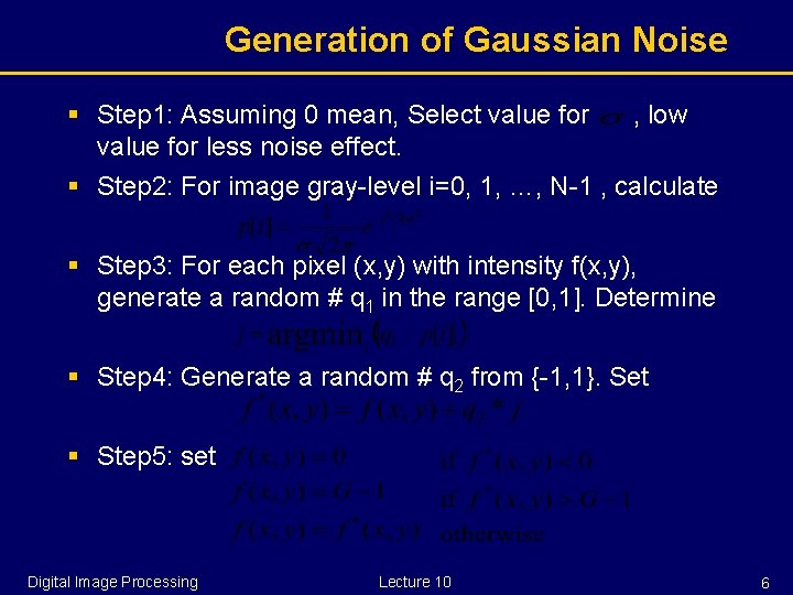
Generation of Gaussian Noise § Step 1: Assuming 0 mean, Select value for , low value for less noise effect. § Step 2: For image gray-level i=0, 1, …, N-1 , calculate § Step 3: For each pixel (x, y) with intensity f(x, y), generate a random # q 1 in the range [0, 1]. Determine § Step 4: Generate a random # q 2 from {-1, 1}. Set § Step 5: set Digital Image Processing Lecture 10 6

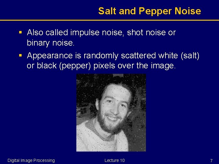
Salt and Pepper Noise § Also called impulse noise, shot noise or binary noise. § Appearance is randomly scattered white (salt) or black (pepper) pixels over the image. Digital Image Processing Lecture 10 7

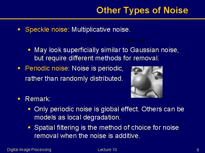
Other Types of Noise § Speckle noise: Multiplicative noise. § May look superficially similar to Gaussian noise, but require different methods for removal. § Periodic noise: Noise is periodic, rather than randomly distributed. § Remark: § Only periodic noise is global effect. Others can be models as local degradation. § Spatial filtering is the method of choice for noise removal when the noise is additive. Digital Image Processing Lecture 10 8

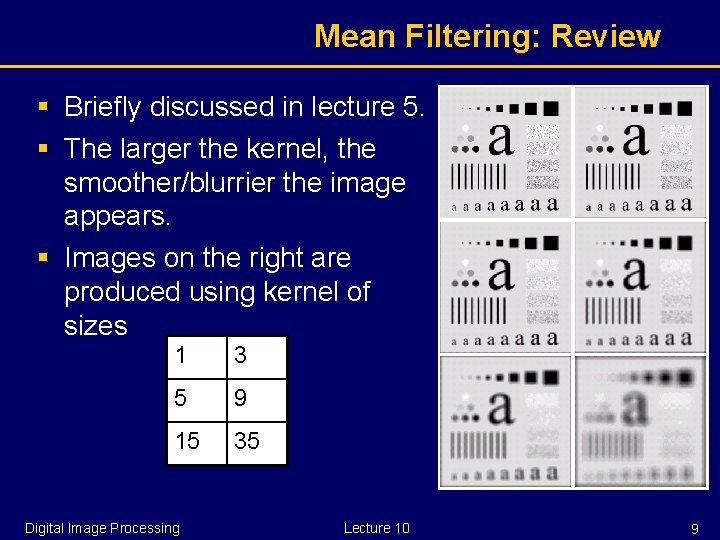
Mean Filtering: Review § Briefly discussed in lecture 5. § The larger the kernel, the smoother/blurrier the image appears. § Images on the right are produced using kernel of sizes 1 3 5 9 15 35 Digital Image Processing Lecture 10 9

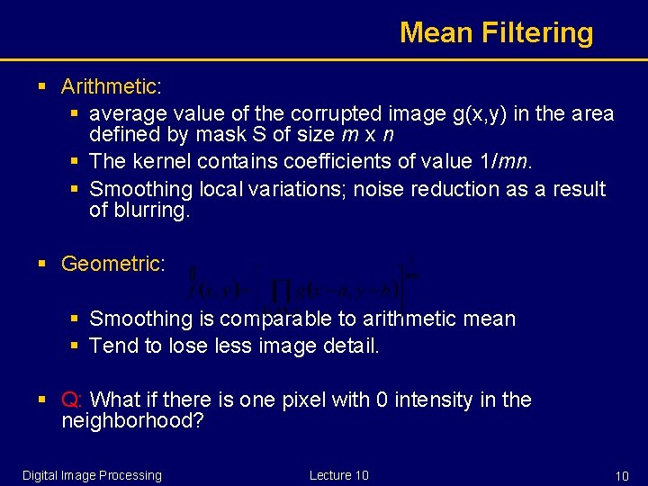
Mean Filtering § Arithmetic: § average value of the corrupted image g(x, y) in the area defined by mask S of size m x n § The kernel contains coefficients of value 1/mn. § Smoothing local variations; noise reduction as a result of blurring. § Geometric: § Smoothing is comparable to arithmetic mean § Tend to lose less image detail. § Q: What if there is one pixel with 0 intensity in the neighborhood? Digital Image Processing Lecture 10 10

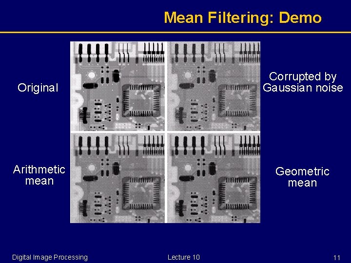
Mean Filtering: Demo Original Corrupted by Gaussian noise Arithmetic mean Geometric mean Digital Image Processing Lecture 10 11

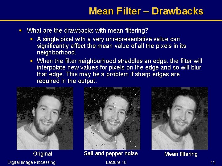
Mean Filter – Drawbacks § What are the drawbacks with mean filtering? § A single pixel with a very unrepresentative value can significantly affect the mean value of all the pixels in its neighborhood. § When the filter neighborhood straddles an edge, the filter will interpolate new values for pixels on the edge and so will blur that edge. This may be a problem if sharp edges are required in the output. Original Digital Image Processing Salt and pepper noise Lecture 10 Mean filtering 12

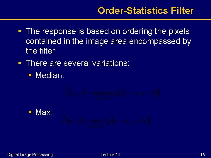
Order-Statistics Filter § The response is based on ordering the pixels contained in the image area encompassed by the filter. § There are several variations: § Median: § Max: Digital Image Processing Lecture 10 13

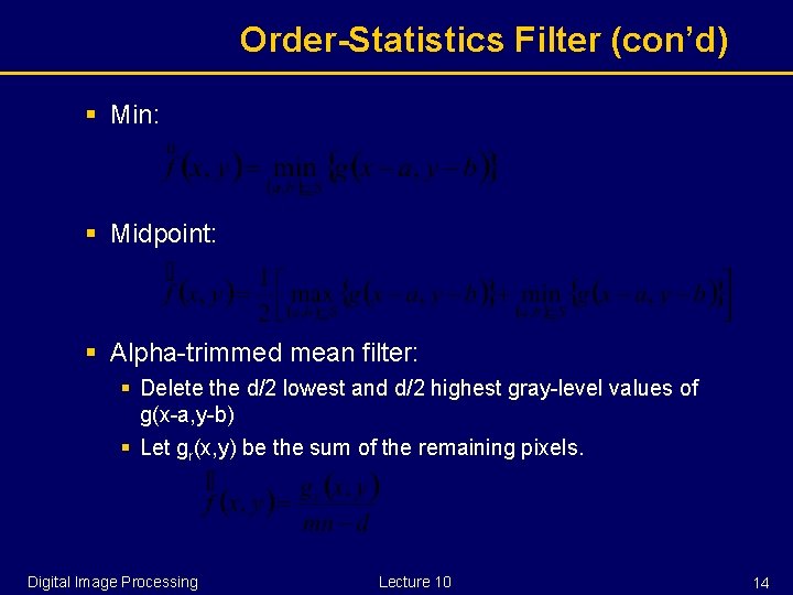
Order-Statistics Filter (con’d) § Min: § Midpoint: § Alpha-trimmed mean filter: § Delete the d/2 lowest and d/2 highest gray-level values of g(x-a, y-b) § Let gr(x, y) be the sum of the remaining pixels. Digital Image Processing Lecture 10 14

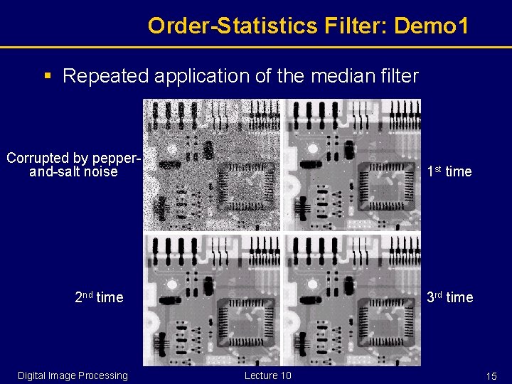
Order-Statistics Filter: Demo 1 § Repeated application of the median filter Corrupted by pepperand-salt noise 1 st time 2 nd time Digital Image Processing 3 rd time Lecture 10 15

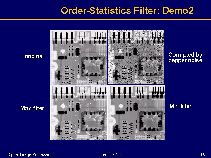
Order-Statistics Filter: Demo 2 Corrupted by pepper noise original Max filter Digital Image Processing ? ? Lecture 10 Min filter 16

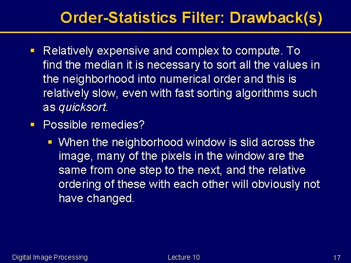
Order-Statistics Filter: Drawback(s) § Relatively expensive and complex to compute. To find the median it is necessary to sort all the values in the neighborhood into numerical order and this is relatively slow, even with fast sorting algorithms such as quicksort. § Possible remedies? § When the neighborhood window is slid across the image, many of the pixels in the window are the same from one step to the next, and the relative ordering of these with each other will obviously not have changed. Digital Image Processing Lecture 10 17

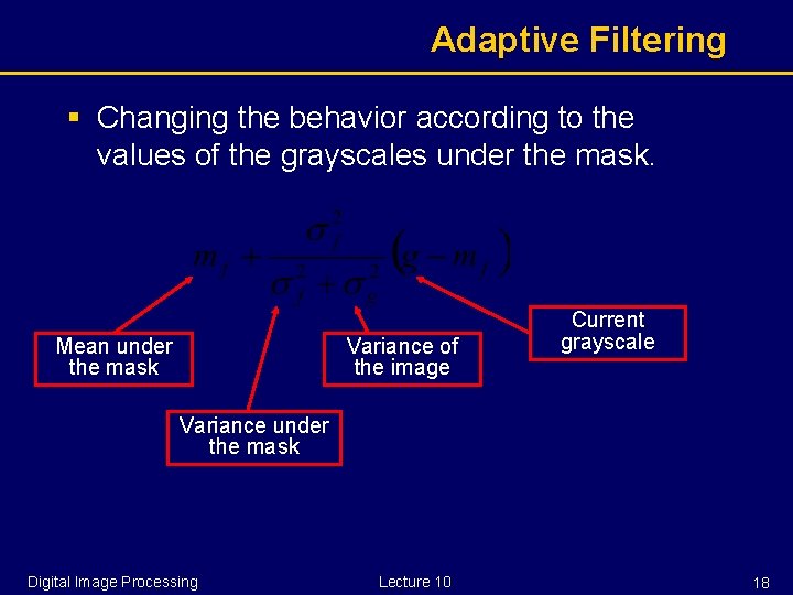
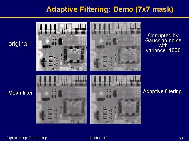
Adaptive Filtering § Changing the behavior according to the values of the grayscales under the mask. Mean under the mask Variance of the image Current grayscale Variance under the mask Digital Image Processing Lecture 10 18

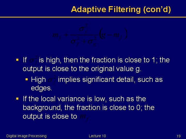
Adaptive Filtering (con’d) § If is high, then the fraction is close to 1; the output is close to the original value g. § High implies significant detail, such as edges. § If the local variance is low, such as the background, the fraction is close to 0; the output is close to Digital Image Processing Lecture 10 19

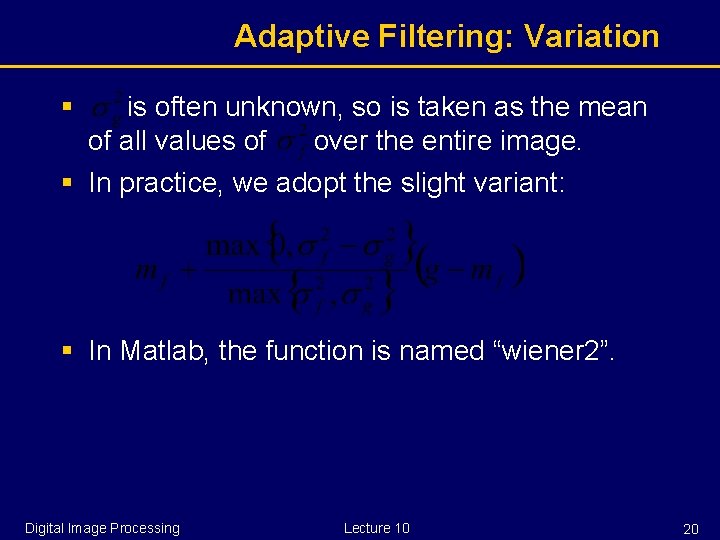
Adaptive Filtering: Variation § is often unknown, so is taken as the mean of all values of over the entire image. § In practice, we adopt the slight variant: § In Matlab, the function is named “wiener 2”. Digital Image Processing Lecture 10 20

Adaptive Filtering: Demo (7 x 7 mask) Corrupted by Gaussian noise with variance=1000 original Adaptive filtering Mean filter Digital Image Processing Lecture 10 21

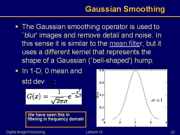
Gaussian Smoothing § The Gaussian smoothing operator is used to `blur' images and remove detail and noise. In this sense it is similar to the mean filter, but it uses a different kernel that represents the shape of a Gaussian (`bell-shaped') hump. § In 1 -D, 0 mean and std dev : We have seen this in filtering in frequency domain Digital Image Processing Lecture 10 22

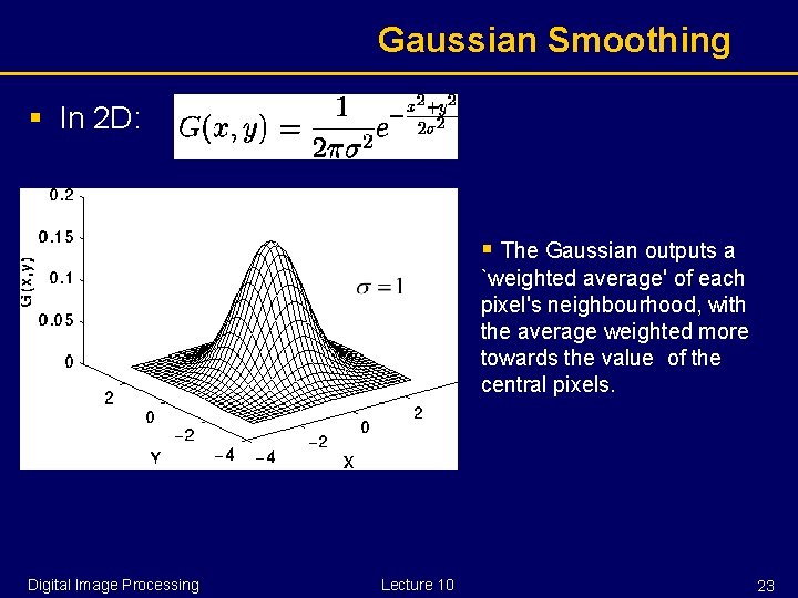
Gaussian Smoothing § In 2 D: § The Gaussian outputs a `weighted average' of each pixel's neighbourhood, with the average weighted more towards the value of the central pixels. Digital Image Processing Lecture 10 23

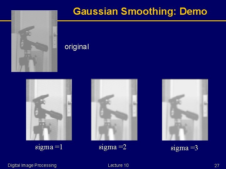
Gaussian Smoothing § The only parameter is (sigma), which is the standard deviation. This value controls the degree of smoothing. § as this parameter goes up, more pixels in the neighborhood are involved in “averaging”, § the image gets more blurred, and § noise is more effectively suppressed Digital Image Processing Lecture 10 24

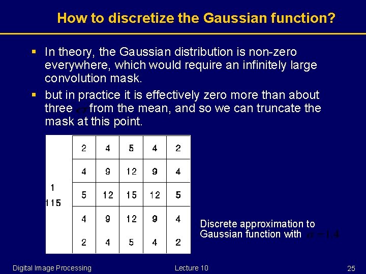
How to discretize the Gaussian function? § In theory, the Gaussian distribution is non-zero everywhere, which would require an infinitely large convolution mask. § but in practice it is effectively zero more than about three from the mean, and so we can truncate the mask at this point. Discrete approximation to Gaussian function with Digital Image Processing Lecture 10 25

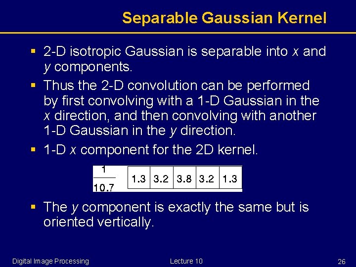
Separable Gaussian Kernel § 2 -D isotropic Gaussian is separable into x and y components. § Thus the 2 -D convolution can be performed by first convolving with a 1 -D Gaussian in the x direction, and then convolving with another 1 -D Gaussian in the y direction. § 1 -D x component for the 2 D kernel. § The y component is exactly the same but is oriented vertically. Digital Image Processing Lecture 10 26

Gaussian Smoothing: Demo original sigma =1 Digital Image Processing sigma =2 Lecture 10 sigma =3 27