Histograms Histogram Equalization Properties of histograms Integrated optical

Histograms Histogram Equalization

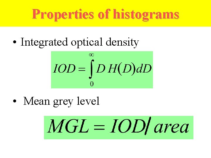
Properties of histograms • Integrated optical density • Mean grey level

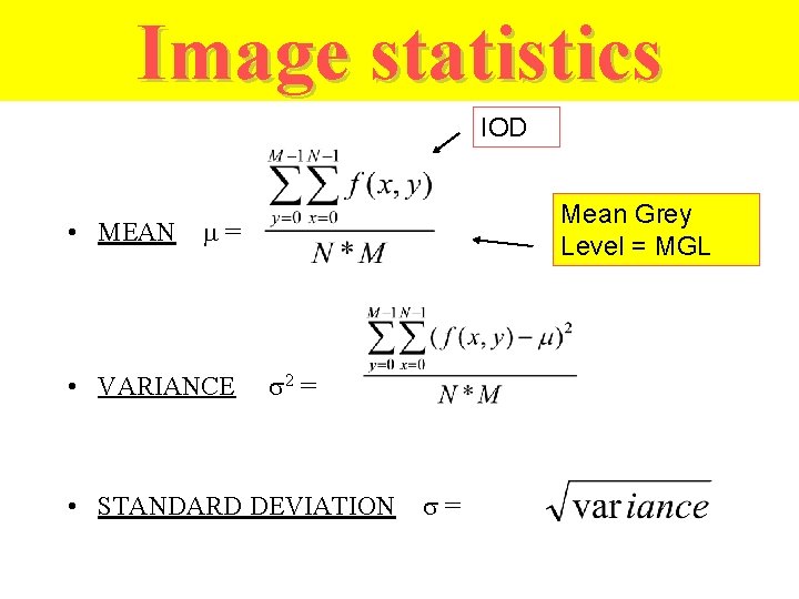
Image statistics IOD Mean Grey Level = MGL • MEAN = • VARIANCE 2 = • STANDARD DEVIATION =

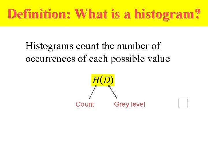
Definition: What is a histogram? Histograms count the number of occurrences of each possible value Count Grey level

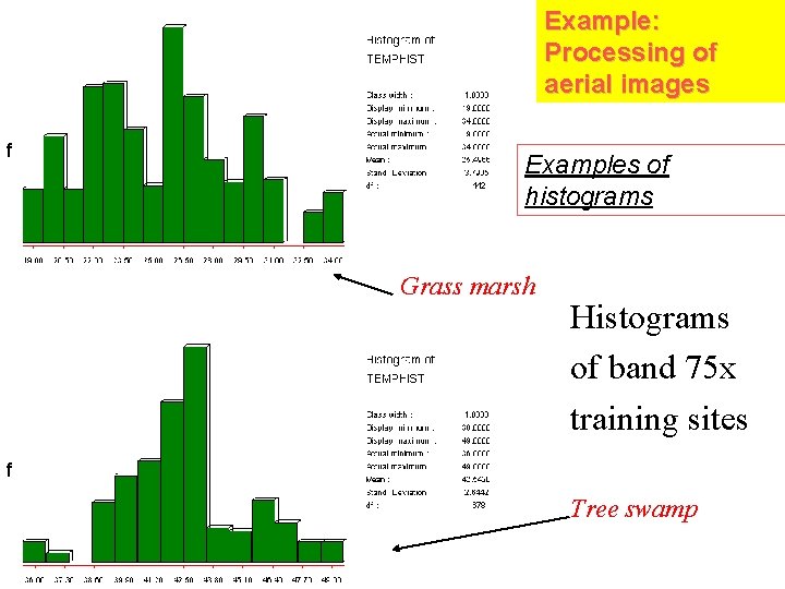
Example: Processing of aerial images Examples of histograms Grass marsh Histograms of band 75 x training sites Tree swamp

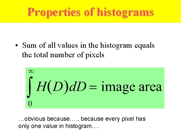
Properties of histograms • Sum of all values in the histogram equals the total number of pixels …obvious because…. . because every pixel has only one value in histogram….

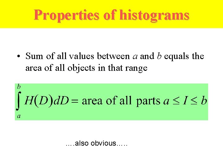
Properties of histograms • Sum of all values between a and b equals the area of all objects in that range …. also obvious…. .

What are the Applications of Histograms? u Image Equalization u. Image Enhancement u. Adjusting Camera Parameters u. Histogram Normalization u. Logarithmic Contrast Enhancement u. Log histogramming for edge detection

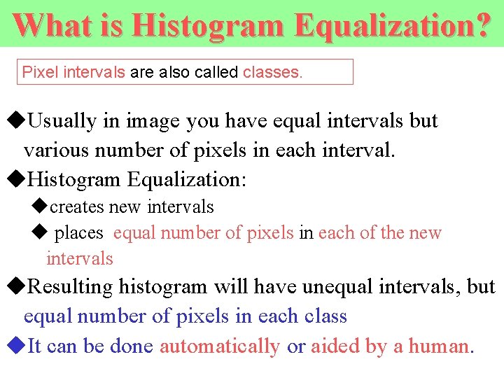
What is Histogram Equalization? Pixel intervals are also called classes. u. Usually in image you have equal intervals but various number of pixels in each interval. u. Histogram Equalization: ucreates new intervals u places equal number of pixels in each of the new intervals u. Resulting histogram will have unequal intervals, but equal number of pixels in each class u. It can be done automatically or aided by a human.

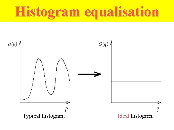
Histogram equalisation Typical histogram Ideal histogram

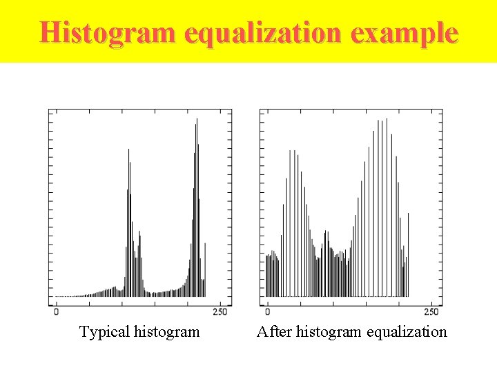
Histogram equalization example Typical histogram After histogram equalization

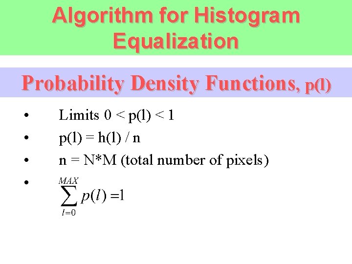
Algorithm for Histogram Equalization Probability Density Functions, p(l) • • Limits 0 < p(l) < 1 p(l) = h(l) / n n = N*M (total number of pixels)

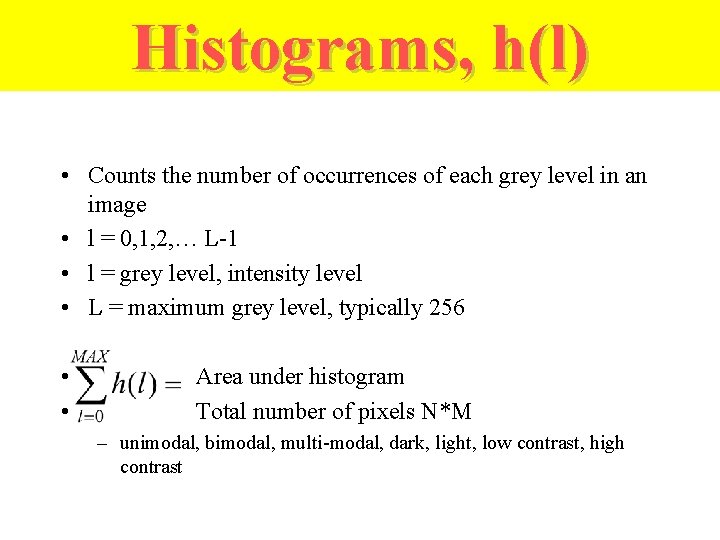
Histograms, h(l) • Counts the number of occurrences of each grey level in an image • l = 0, 1, 2, … L-1 • l = grey level, intensity level • L = maximum grey level, typically 256 • • Area under histogram Total number of pixels N*M – unimodal, bimodal, multi-modal, dark, light, low contrast, high contrast

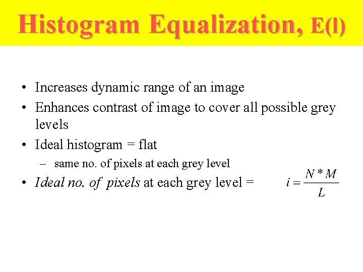
Histogram Equalization, E(l) • Increases dynamic range of an image • Enhances contrast of image to cover all possible grey levels • Ideal histogram = flat – same no. of pixels at each grey level • Ideal no. of pixels at each grey level =

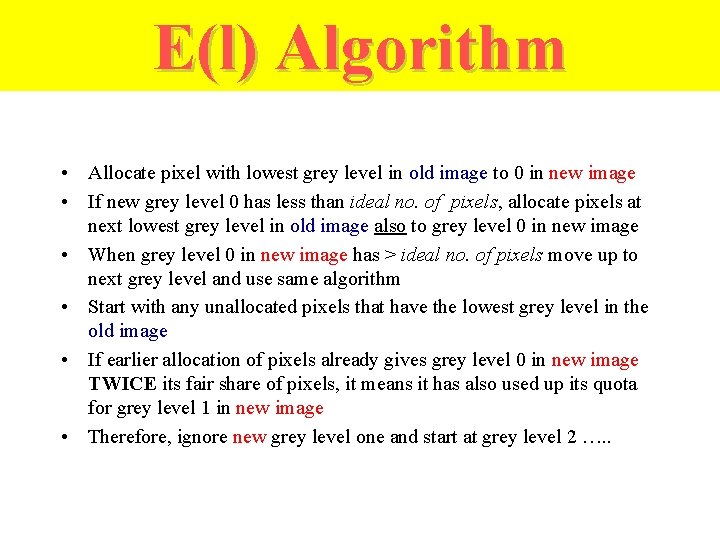
E(l) Algorithm • Allocate pixel with lowest grey level in old image to 0 in new image • If new grey level 0 has less than ideal no. of pixels, allocate pixels at next lowest grey level in old image also to grey level 0 in new image • When grey level 0 in new image has > ideal no. of pixels move up to next grey level and use same algorithm • Start with any unallocated pixels that have the lowest grey level in the old image • If earlier allocation of pixels already gives grey level 0 in new image TWICE its fair share of pixels, it means it has also used up its quota for grey level 1 in new image • Therefore, ignore new grey level one and start at grey level 2 …. .

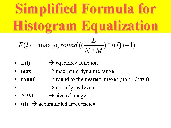
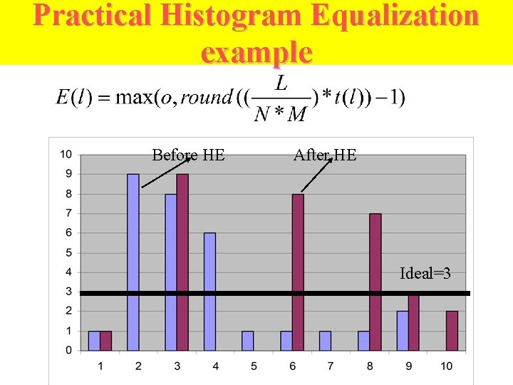
Simplified Formula for Histogram Equalization • • • E(l) equalized function maximum dynamic range round to the nearest integer (up or down) L no. of grey levels N*M size of image t(l) accumulated frequencies

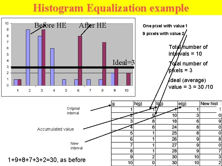
Practical Histogram Equalization example Before HE After HE Ideal=3

Histogram Equalization example Before HE After HE One pixel with value 1 9 pixels with value 2 Total number of intervals = 10 Ideal=3 Total number of pixels = 3 Ideal (average) value = 30 /10 Original interval Accumulated value New interval 1+9+8+7+3+2=30, as before 1

Where is Histogram Equalization Used? urobot vision, u photographics, uaerial images

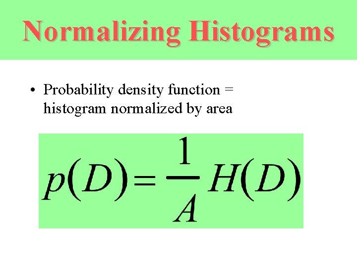
Normalizing Histograms • Probability density function = histogram normalized by area

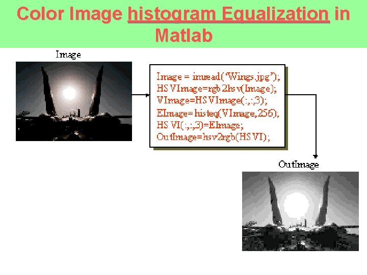
Color Image histogram Equalization in Matlab

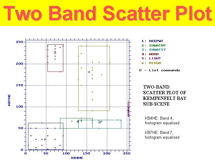
Two Band Scatter Plot

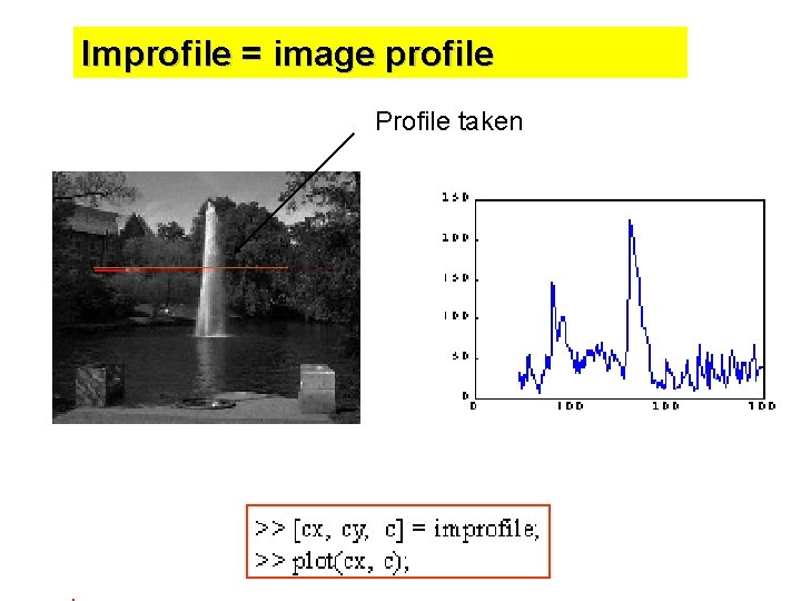
Improfile = image profile Profile taken

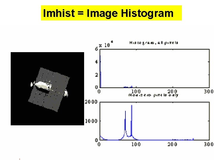
Imhist = Image Histogram

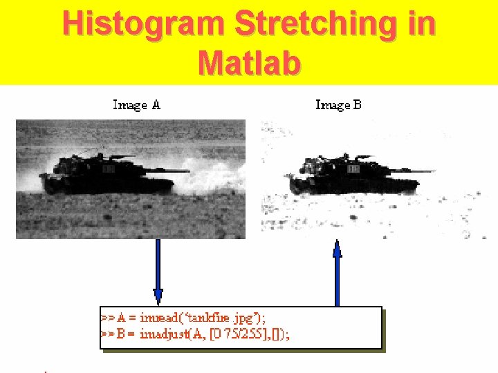
Histogram Stretching in Matlab

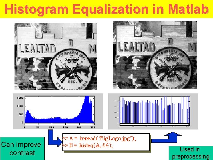
Histogram Equalization in Matlab Can improve contrast Used in preprocessing

Application: Adjusting Camera Parameters • Too bright - lots of pixels at 255 (or max) • Too dark - lots of pixels at 0 • Gain too low - not enough of the range used Example of image enhancement

Application: Image Segmentation • Can be used to separate bright objects from dark background (or vice versa)

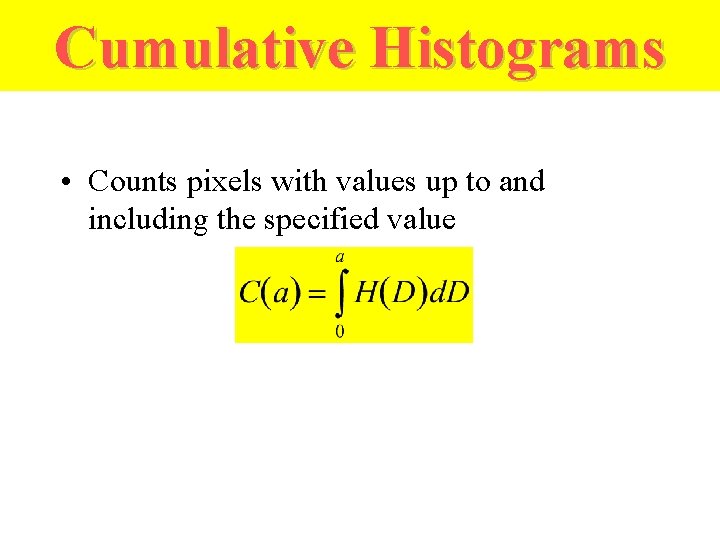
Cumulative Histograms • Counts pixels with values up to and including the specified value

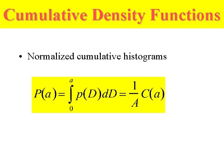
Cumulative Density Functions • Normalized cumulative histograms

IMAGE ENHANCEMENT

IMAGE ENHANCEMENT u. Due to the fact that original pixel values are integer values, and that frequency of the values varies with each class, the result will be an actual number of pixels in each class which only approximates the equalized percentage u. Alternative explanation which incorporates probability and a transformation function: unote the difference in the two histograms, original and equalized

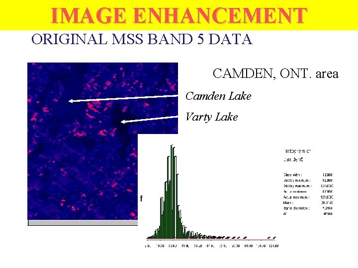
IMAGE ENHANCEMENT ORIGINAL MSS BAND 5 DATA CAMDEN, ONT. area Camden Lake Varty Lake

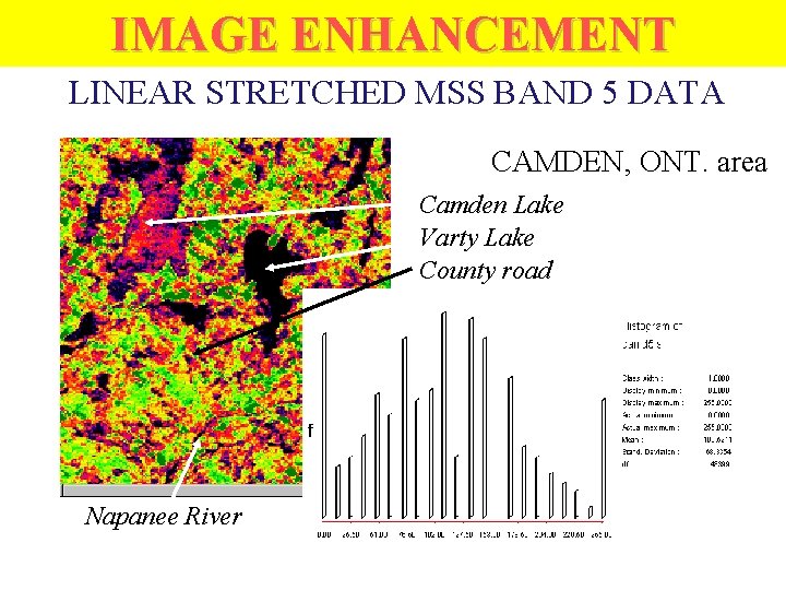
IMAGE ENHANCEMENT LINEAR STRETCHED MSS BAND 5 DATA CAMDEN, ONT. area Camden Lake Varty Lake County road Napanee River

IMAGE ENHANCEMENT SPATIAL FILTERING • Spatial frequency: “The number of changes in brightness value per unit distance for any particular part of an image” (Jensen) – Few changes? Low frequency – Many changes? High frequency

IMAGE ENHANCEMENT • The principles? Pixel values along a single scan line can be represented by a complex curve which comprises many simple curves, each with its own constant wavelength • The complex curve can be separated into its component wavelengths by mathematical process of filtering

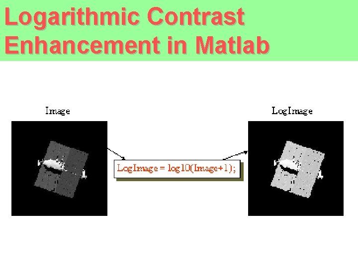
Logarithmic Contrast Enhancement in Matlab

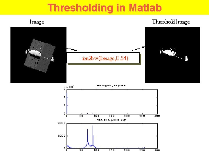
Thresholding in Matlab

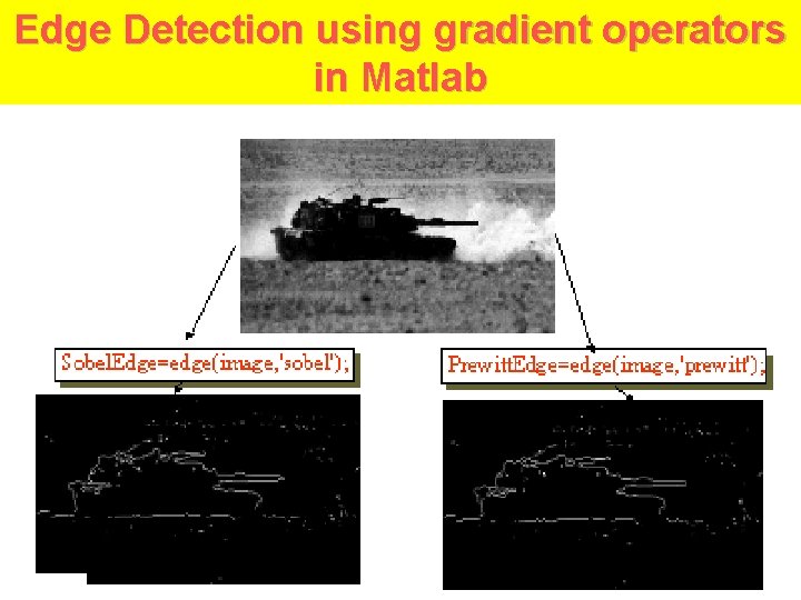
Edge Detection using gradient operators in Matlab

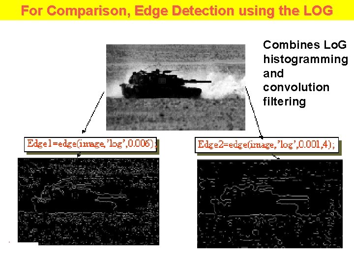
For Comparison, Edge Detection using the LOG Combines Lo. G histogramming and convolution filtering

POINT OPERATIONS • Operates on ONLY 1 pixel at a time without considering neighboring values • Thresholding • Contrast stretching • Temporal image smoothing • Image difference • Color adjustment or selection

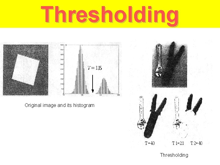
Thresholding • Creates binary image from grayscale image • Image histogram • Determining threshold

Temporal smoothing • Noisy images, e. g. pictures from the moon • Several frames of the same scene • Take average of the same pixel value over time • Standard deviation of noise decreases on averaging

Image difference over time • Static camera is assumed • Compute I(t) - I(t+dt) • Threshold to eliminate small differences • Still scene ==> Nothing in difference • Moving object ==> object detected before & after motion

Color adjustment/selection • • Hue, saturation, intensity Red, green, blue Selecting sky Selecting grass

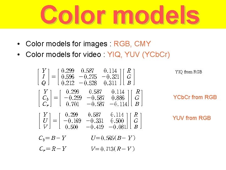
Color models • Color models for images : RGB, CMY • Color models for video : YIQ, YUV (YCb. Cr) YIQ from RGB YCb. Cr from RGB YUV from RGB

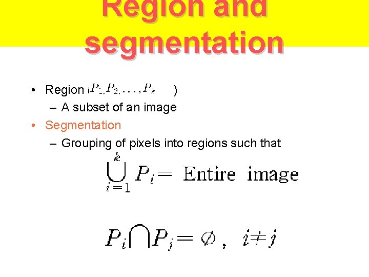
Region and segmentation • Region ( ) – A subset of an image • Segmentation – Grouping of pixels into regions such that

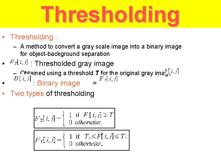
Thresholding • Thresholding : – A method to convert a gray scale image into a binary image for object-background separation • : Thresholded gray image – Obtained using a threshold T for the original gray image • : Binary image = • Two types of thresholding

Thresholding Original image and its histogram Thresholding

Sources • Maja Mataric • Dodds, Harvey Mudd College • Damien Blond • • Alim Fazal Tory Richard Jim Gast Bryan S. Morse Gerald Mc. Grath Vanessa S. Blake Matt Roach • Bryan S. Morse • Many WWW sources • Anup Basu, Ph. D. Professor, Dept of Computing Sc. University of Alberta • Professor Kim, KAIST • H. Schultz, Computer science, University of Massachusetts, Web Site: www-edlab. cs. umass/cs 570 • Many sources of slides from Internet http: //www. cheng. cam. ac. uk/seminars/imagepro/

Sources • 533 Text book • http: //sern. ucalgary. ca/courses/CPSC/533/W 99/ presentations/L 2_24 A_Lee_Wang/ http: //sern. ucalgary. ca/courses/CPSC/533/W 99/ presentations/L 1_24 A_Kaasten_Steller_Hoang/main. htm http: //sern. ucalgary. ca/courses/CPSC/533/W 99/ presentations/L 1_24_Schebywolok/index. html http: //sern. ucalgary. ca/courses/CPSC/533/W 99/ presentations/L 2_24 B_Doering_Grenier/ • http: //www. geocities. com/So. Ho/Museum/3828/ optical. html • http: //members. spree. com/fun. Ngames/katbug/

Noise Reduction

Image Enhancement • • • Brightness control Contrast enhancement Noise reduction Edge enhancement Zooming

Objectives • What is noise? • How is noise reduction performed? – Noise reduction from first principles – Neighbourhood operators • linear filters (low pass, high pass) • non-linear filters (median)

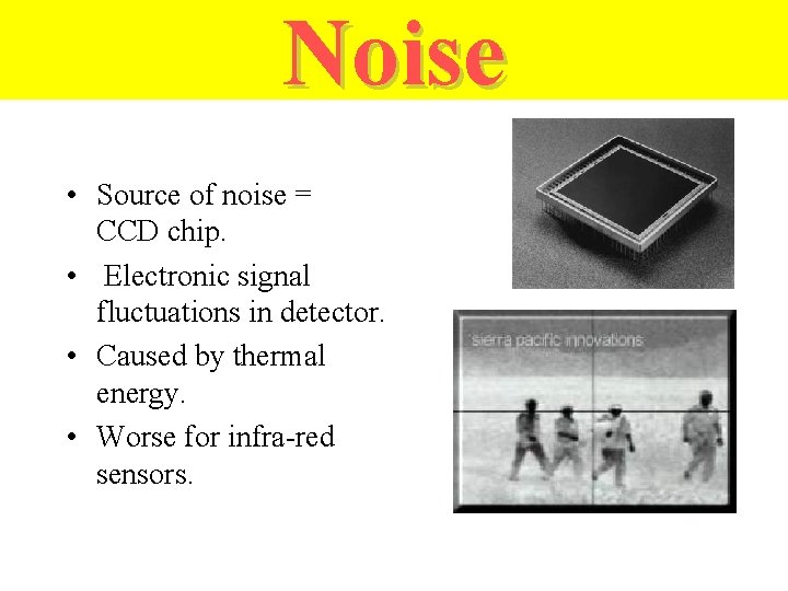
Noise • Source of noise = CCD chip. • Electronic signal fluctuations in detector. • Caused by thermal energy. • Worse for infra-red sensors.

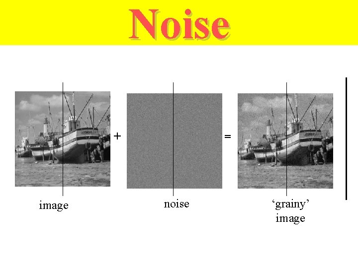
Noise + image = noise ‘grainy’ image

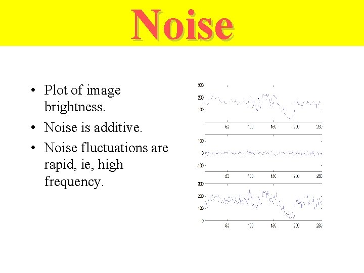
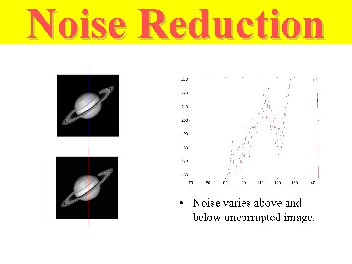
Noise • Plot of image brightness. • Noise is additive. • Noise fluctuations are rapid, ie, high frequency.

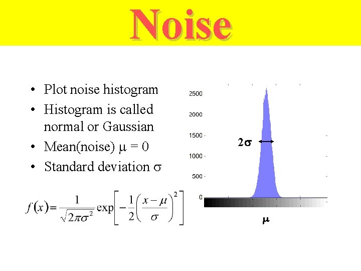
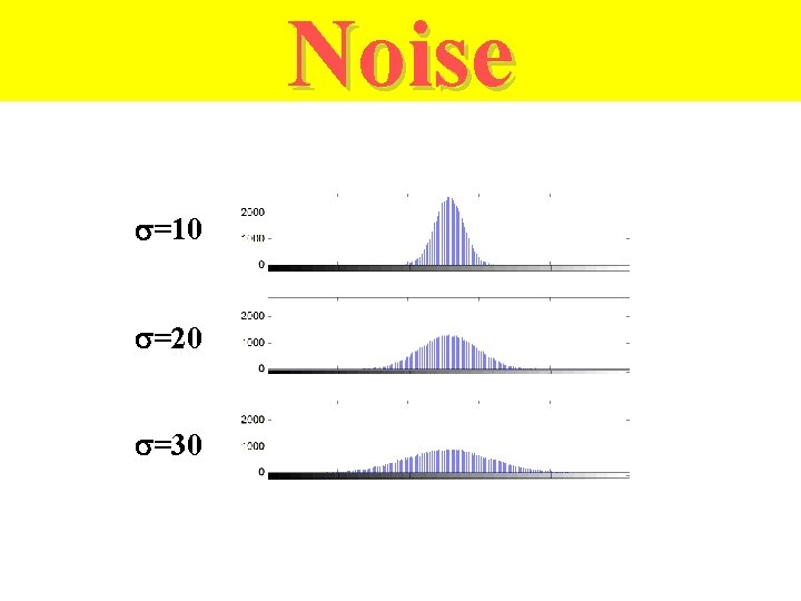
Noise • Plot noise histogram • Histogram is called normal or Gaussian • Mean(noise) = 0 • Standard deviation 2

Noise =10 =20 =30

Noise Reduction • Noise varies above and below uncorrupted image.

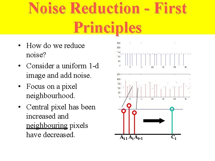
Noise Reduction - First Principles • How do we reduce noise? • Consider a uniform 1 -d image and add noise. • Focus on a pixel neighbourhood. • Central pixel has been increased and neighbouring pixels have decreased. Ai-1 Ai Ai+1 Ci

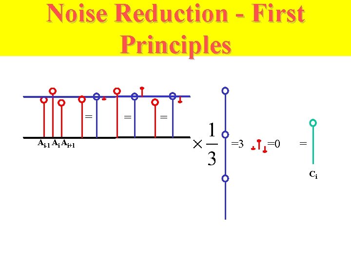
Noise Reduction - First Principles = Ai-1 Ai Ai+1 = = =3 =0 = Ci

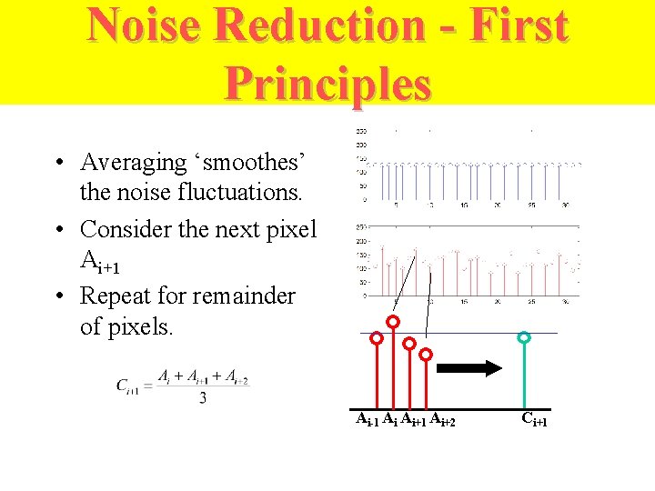
Noise Reduction - First Principles • Averaging ‘smoothes’ the noise fluctuations. • Consider the next pixel Ai+1 • Repeat for remainder of pixels. Ai-1 Ai Ai+1 Ai+2 Ci+1

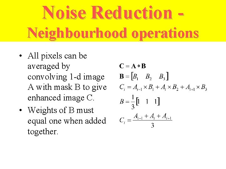
Noise Reduction Neighbourhood operations • All pixels can be averaged by convolving 1 -d image A with mask B to give enhanced image C. • Weights of B must equal one when added together.

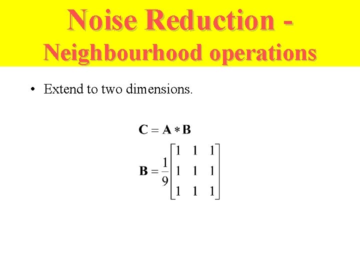
Noise Reduction Neighbourhood operations • Extend to two dimensions.

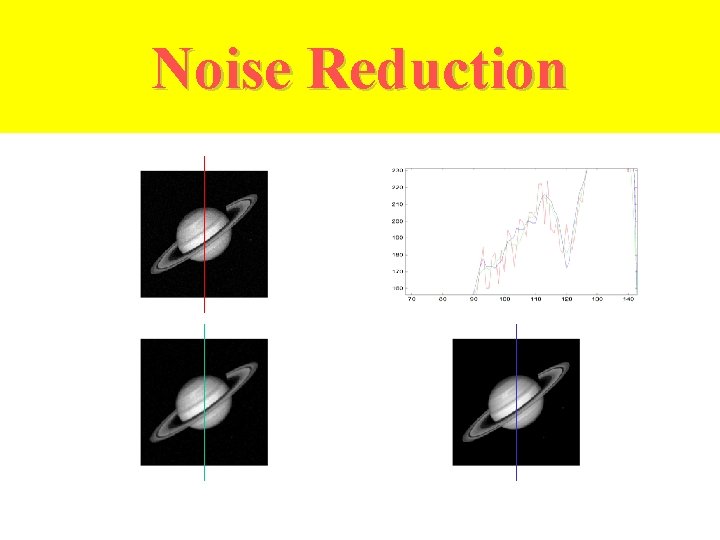
Noise Reduction

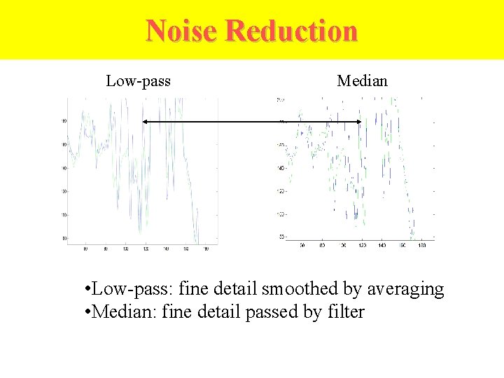
Noise Reduction • Technique relies on high frequency noise fluctuations being ‘blocked’ by filter. Hence, low-pass filter. • Fine detail in image may also be smoothed. • Balance between keeping image fine detail and reducing noise.

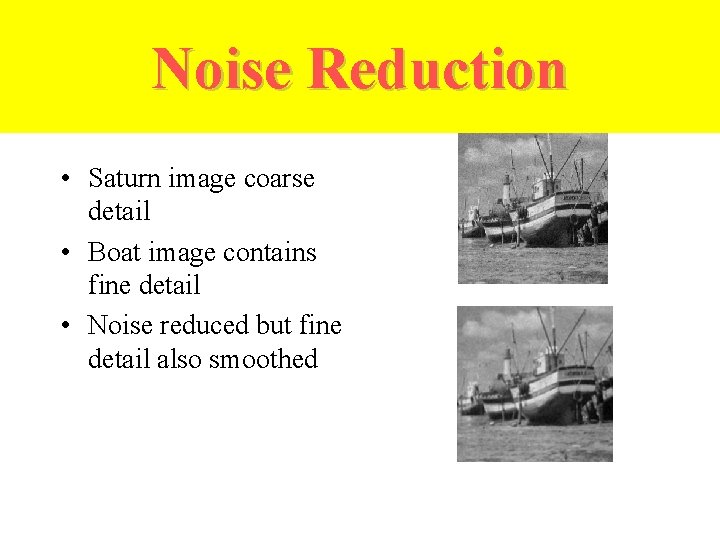
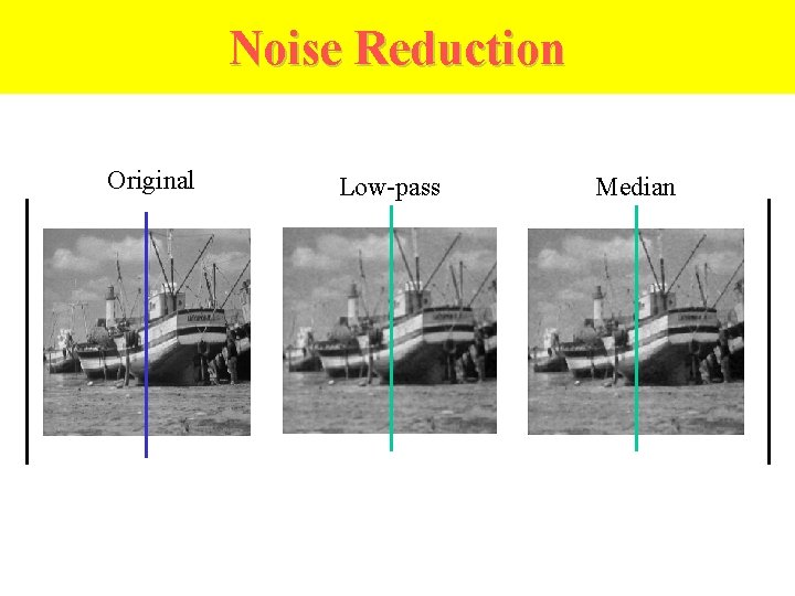
Noise Reduction • Saturn image coarse detail • Boat image contains fine detail • Noise reduced but fine detail also smoothed

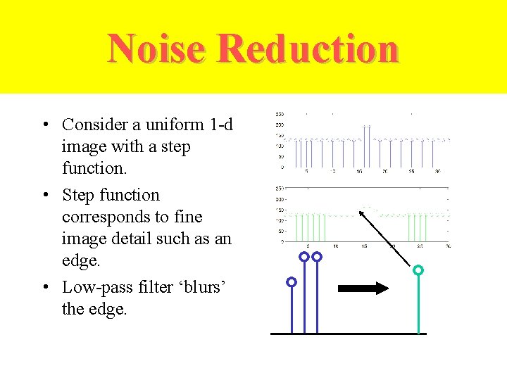
Noise Reduction • Consider a uniform 1 -d image with a step function. • Step function corresponds to fine image detail such as an edge. • Low-pass filter ‘blurs’ the edge.

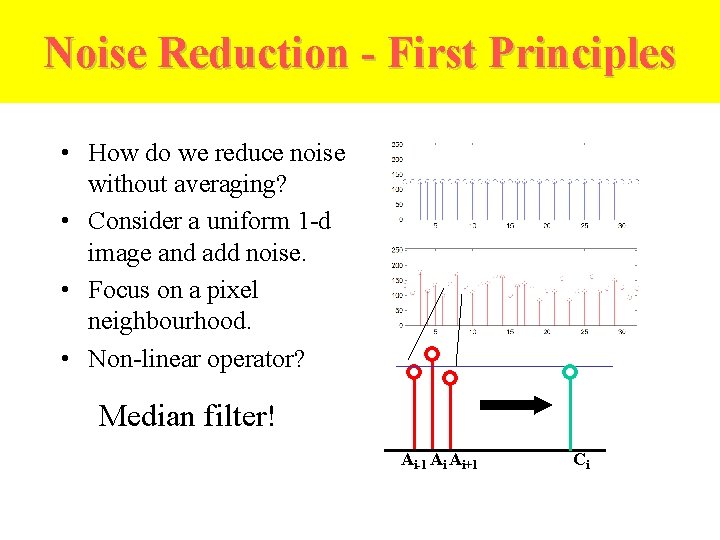
Noise Reduction - First Principles • How do we reduce noise without averaging? • Consider a uniform 1 -d image and add noise. • Focus on a pixel neighbourhood. • Non-linear operator? Median filter! Ai-1 Ai Ai+1 Ci

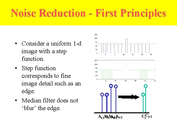
Noise Reduction - First Principles • Consider a uniform 1 -d image with a step function. • Step function corresponds to fine image detail such as an edge. • Median filter does not ‘blur’ the edge. A Ai-1 AAi A i+1 i+2 Ci. Ci+1

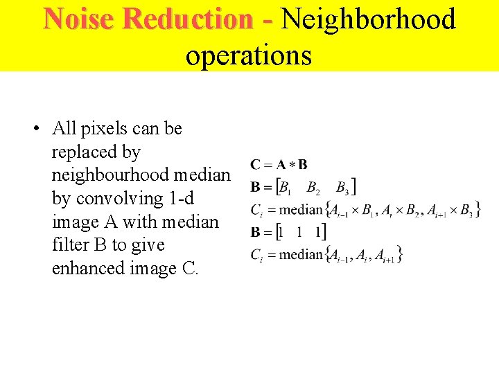
Noise Reduction - Neighborhood operations • All pixels can be replaced by neighbourhood median by convolving 1 -d image A with median filter B to give enhanced image C.

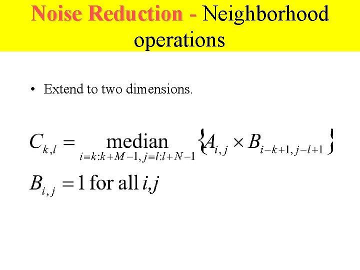
Noise Reduction - Neighborhood operations • Extend to two dimensions.

Noise Reduction Original Low-pass Median

Noise Reduction Low-pass Median • Low-pass: fine detail smoothed by averaging • Median: fine detail passed by filter

Summary • What is noise? – Gaussian distribution • Noise reduction – first principles • Neighbourhood – low-pass – median Conclusion • Averaging pixels corrupted by noise cancels out the noise. • Low-pass can blur image. • Median can retain fine image detail that may be smoothed by averaging.