Go with the Flow Fluid Dynamics Class 3

Go with the Flow! Fluid Dynamics Class 3: Systems of Differential Equations (Part 2)

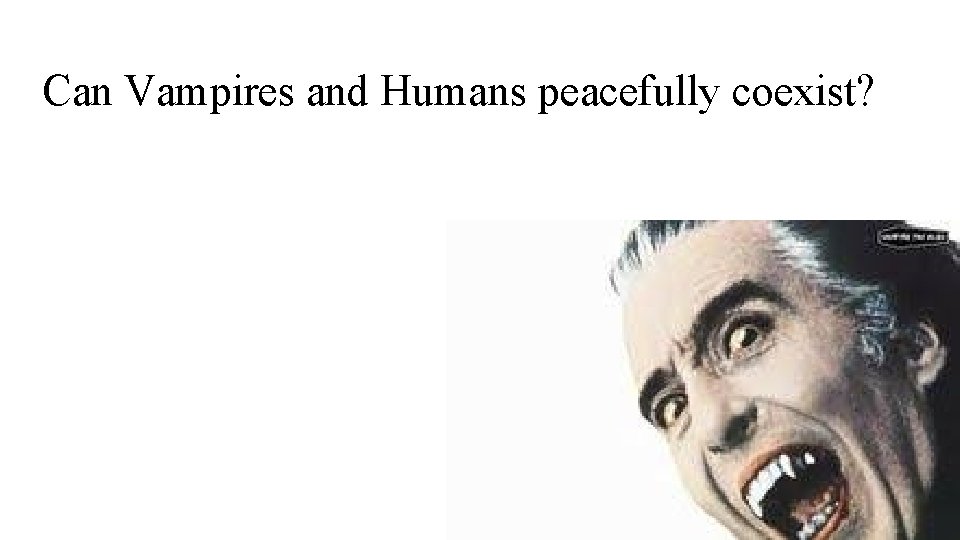
Can Vampires and Humans peacefully coexist?

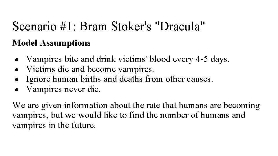
Scenario #1: Bram Stoker's "Dracula" Model Assumptions ● ● Vampires bite and drink victims' blood every 4 -5 days. Victims die and become vampires. Ignore human births and deaths from other causes. Vampires never die. We are given information about the rate that humans are becoming vampires, but we would like to find the number of humans and vampires in the future.

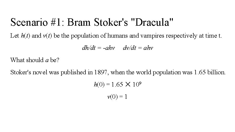
Scenario #1: Bram Stoker's "Dracula" Let h(t) and v(t) be the population of humans and vampires respectively at time t. dh/dt = -ahv dv/dt = ahv What should a be? Stoker's novel was published in 1897, when the world population was 1. 65 billion. h(0) = 1. 65 ✕ 109 v(0) = 1

Coexistence is not possible in scenario #1: Bram Stoker's "Dracula!"

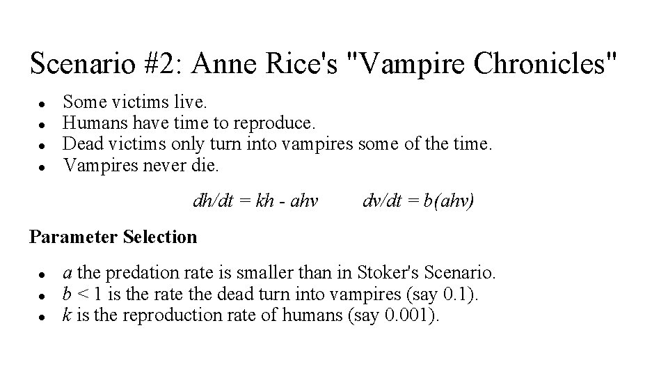
Scenario #2: Anne Rice's "Vampire Chronicles" ● ● Some victims live. Humans have time to reproduce. Dead victims only turn into vampires some of the time. Vampires never die. dh/dt = kh - ahv dv/dt = b(ahv) Parameter Selection ● ● ● a the predation rate is smaller than in Stoker's Scenario. b < 1 is the rate the dead turn into vampires (say 0. 1). k is the reproduction rate of humans (say 0. 001).

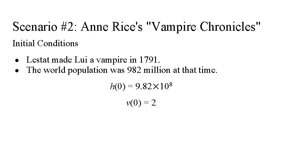
Scenario #2: Anne Rice's "Vampire Chronicles" Initial Conditions ● ● Lestat made Lui a vampire in 1791. The world population was 982 million at that time. h(0) = 9. 82✕ 108 v(0) = 2

Coexistence is not possible in scenario #2: Anne Rice's "Vampire Chronicles!"

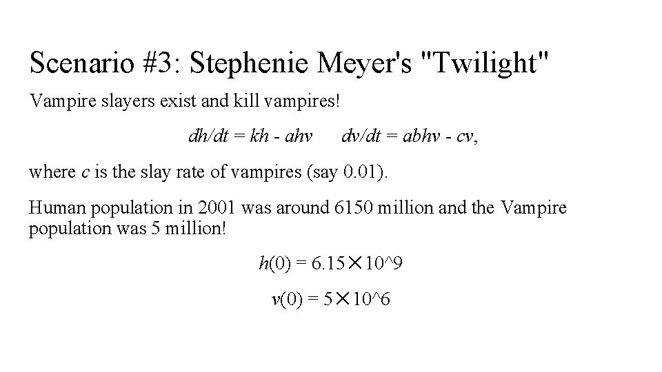
Scenario #3: Stephenie Meyer's "Twilight" Vampire slayers exist and kill vampires! dh/dt = kh - ahv dv/dt = abhv - cv, where c is the slay rate of vampires (say 0. 01). Human population in 2001 was around 6150 million and the Vampire population was 5 million! h(0) = 6. 15✕ 10^9 v(0) = 5✕ 10^6

Coexistence is possible in scenario #3: Stephenie Meyer's "Twilight" series!

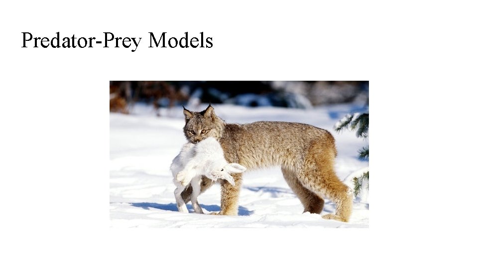
Predator-Prey Models

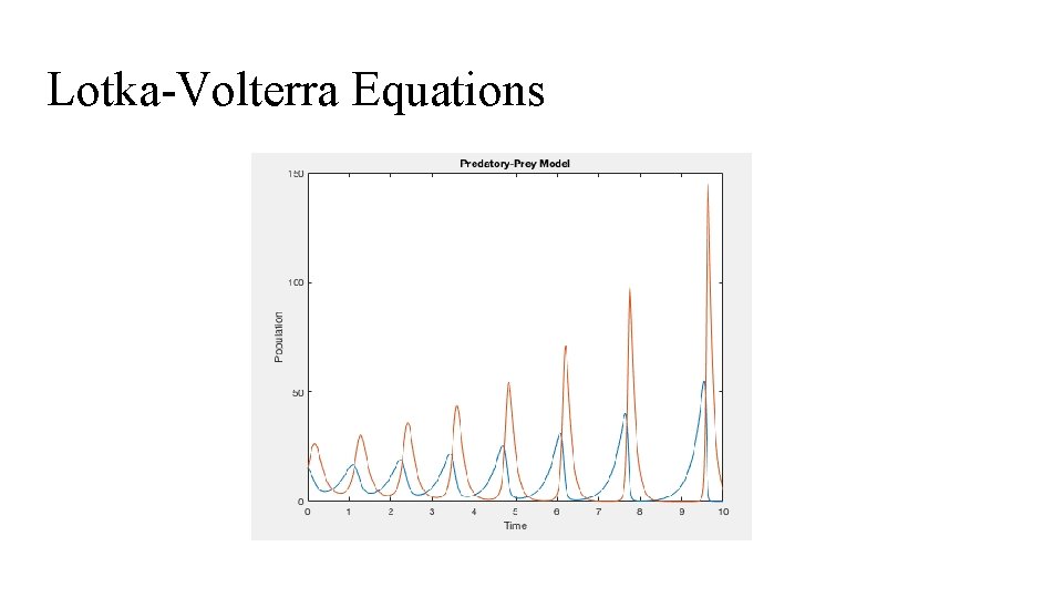
Predator-Prey Models The predator-prey model is a system of differential equations that can also be modeled using Lotka-Volterra equations. Can you think of any examples of species that we may represent using this model?

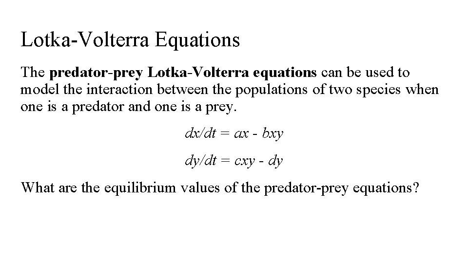
Lotka-Volterra Equations The predator-prey Lotka-Volterra equations can be used to model the interaction between the populations of two species when one is a predator and one is a prey. dx/dt = ax - bxy dy/dt = cxy - dy What are the equilibrium values of the predator-prey equations?

Lotka-Volterra Equations

Predator-Prey Model Practice Research and find two species of animals, one predator and one prey. Make reasonable assumptions and determine how the populations change over time.

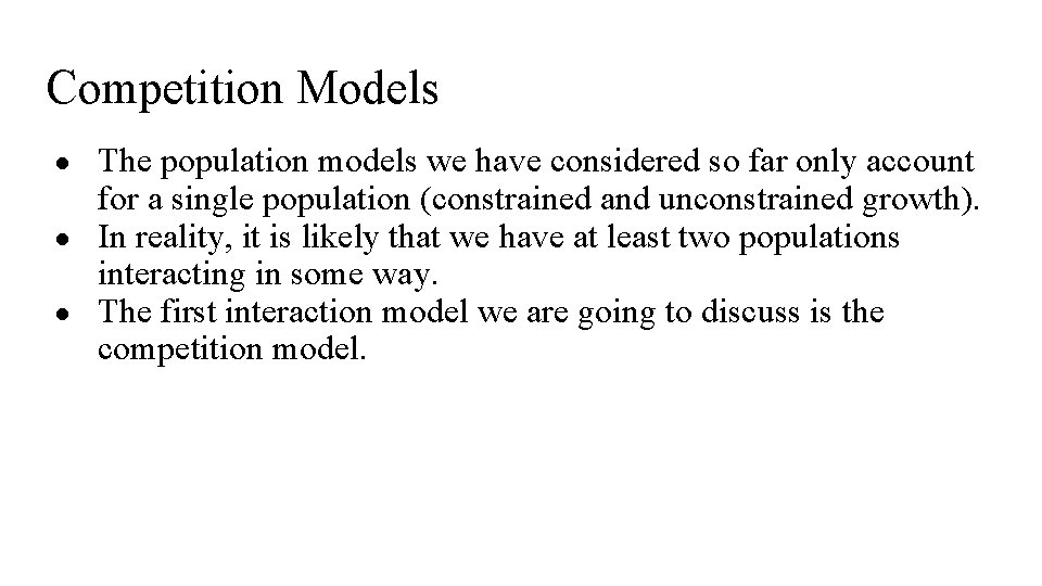
Competition Models ● ● ● The population models we have considered so far only account for a single population (constrained and unconstrained growth). In reality, it is likely that we have at least two populations interacting in some way. The first interaction model we are going to discuss is the competition model.

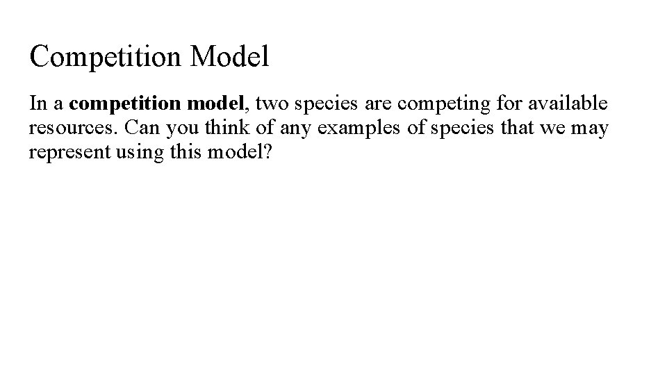
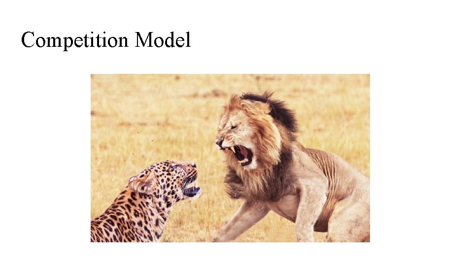
Competition Model In a competition model, two species are competing for available resources. Can you think of any examples of species that we may represent using this model?

Competition Model

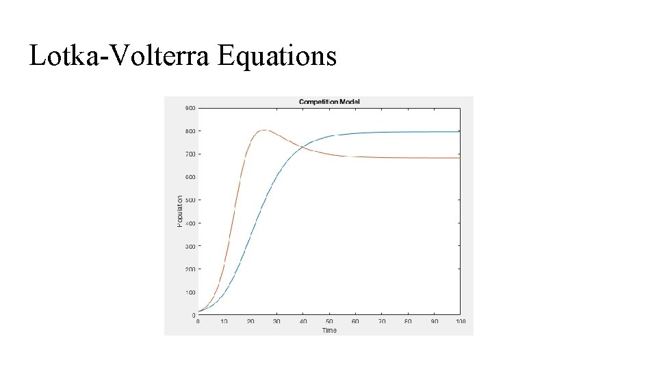
Lotka-Volterra Equations The competitive Lotka-Volterra equations can be used to model the interaction between the populations of two species competing for available resources.

Lotka-Volterra Equations

Competition Model Practice Research and find two species of animals that compete over available resources. Make reasonable assumptions and determine how the populations change over time.

Modeling the Spread of Disease ● Another phenomenon we may want to model is the spread of disease. Take some time to research some major epidemics. ● How might we model the spread of disease?

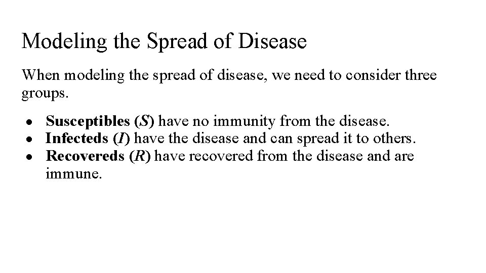
Modeling the Spread of Disease When modeling the spread of disease, we need to consider three groups. ● ● ● Susceptibles (S) have no immunity from the disease. Infecteds (I) have the disease and can spread it to others. Recovereds (R) have recovered from the disease and are immune.

SIR Model In order to model each of these populations, we will consider a system of differential equations called the SIR model.

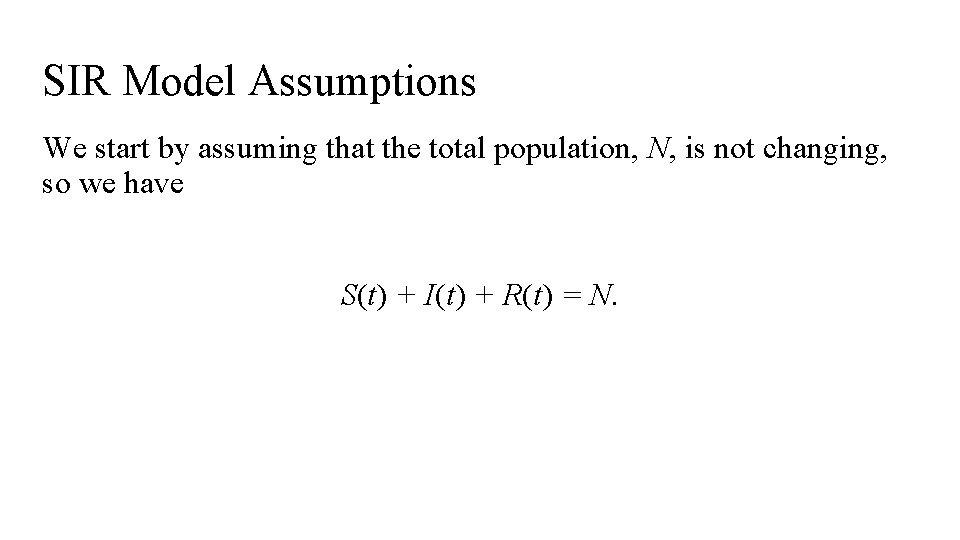
SIR Model Assumptions We start by assuming that the total population, N, is not changing, so we have S(t) + I(t) + R(t) = N.

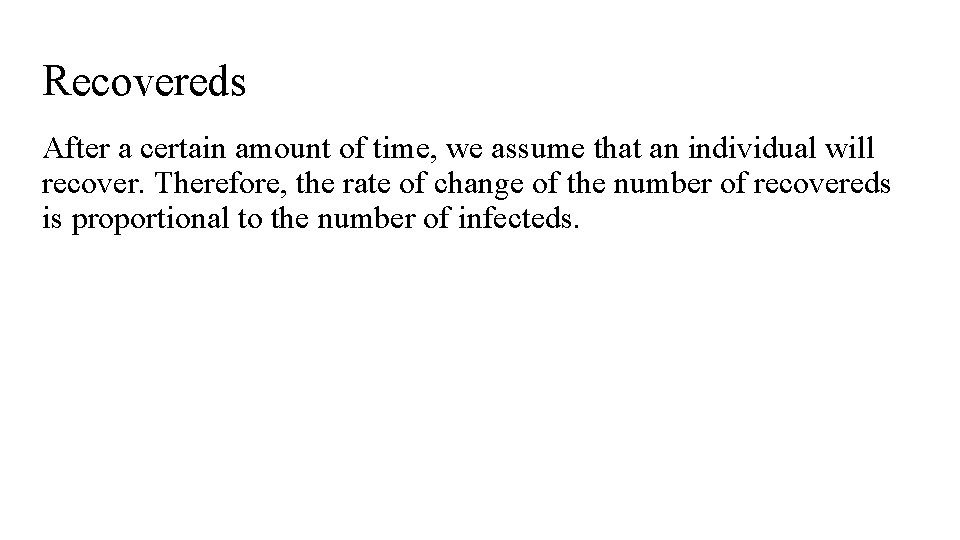
Recovereds After a certain amount of time, we assume that an individual will recover. Therefore, the rate of change of the number of recovereds is proportional to the number of infecteds.

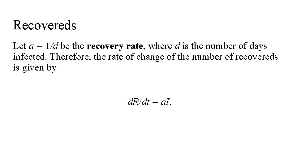
Recovereds Let a = 1/d be the recovery rate, where d is the number of days infected. Therefore, the rate of change of the number of recovereds is given by d. R/dt = a. I.

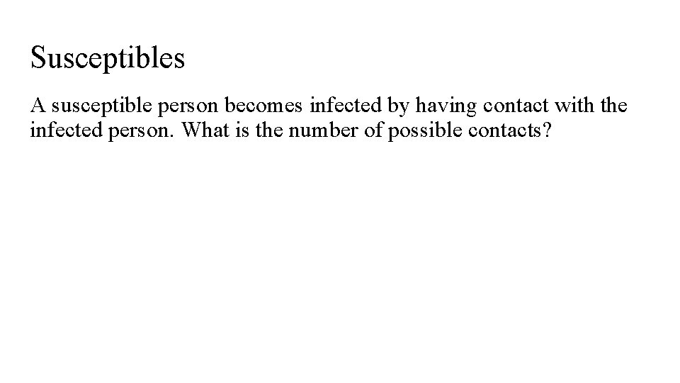
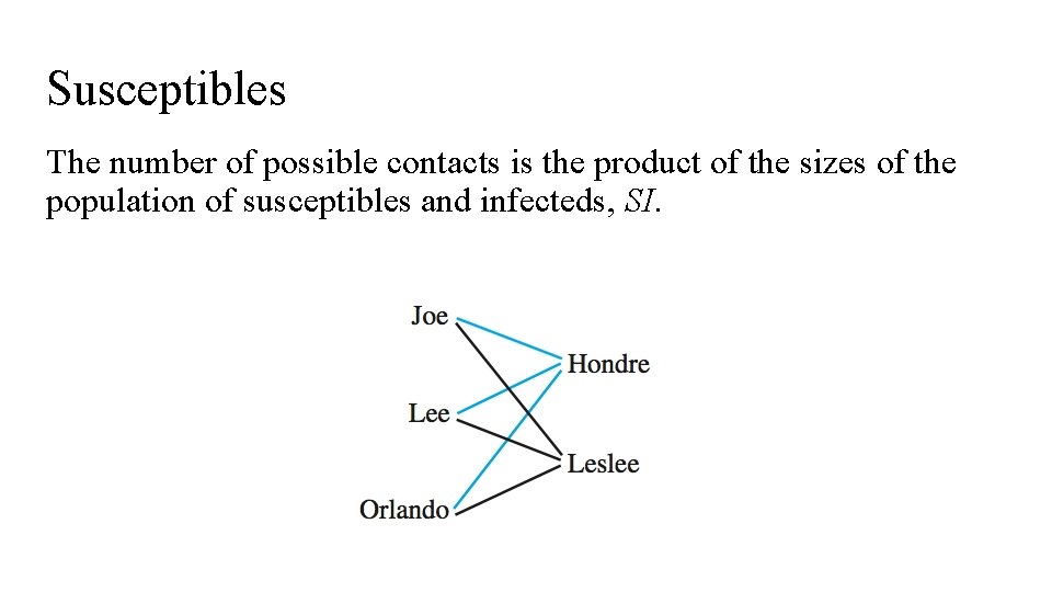
Susceptibles A susceptible person becomes infected by having contact with the infected person. What is the number of possible contacts?

Susceptibles The number of possible contacts is the product of the sizes of the population of susceptibles and infecteds, SI.

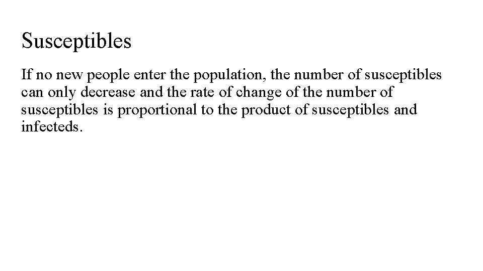
Susceptibles If no new people enter the population, the number of susceptibles can only decrease and the rate of change of the number of susceptibles is proportional to the product of susceptibles and infecteds.

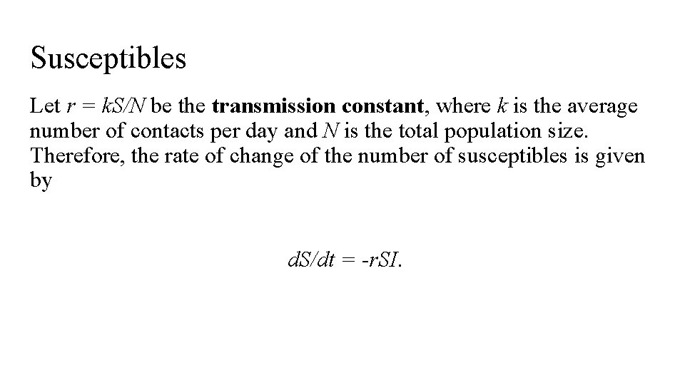
Susceptibles Let r = k. S/N be the transmission constant, where k is the average number of contacts per day and N is the total population size. Therefore, the rate of change of the number of susceptibles is given by d. S/dt = -r. SI.

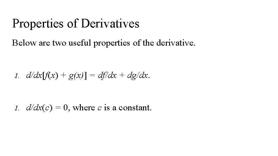
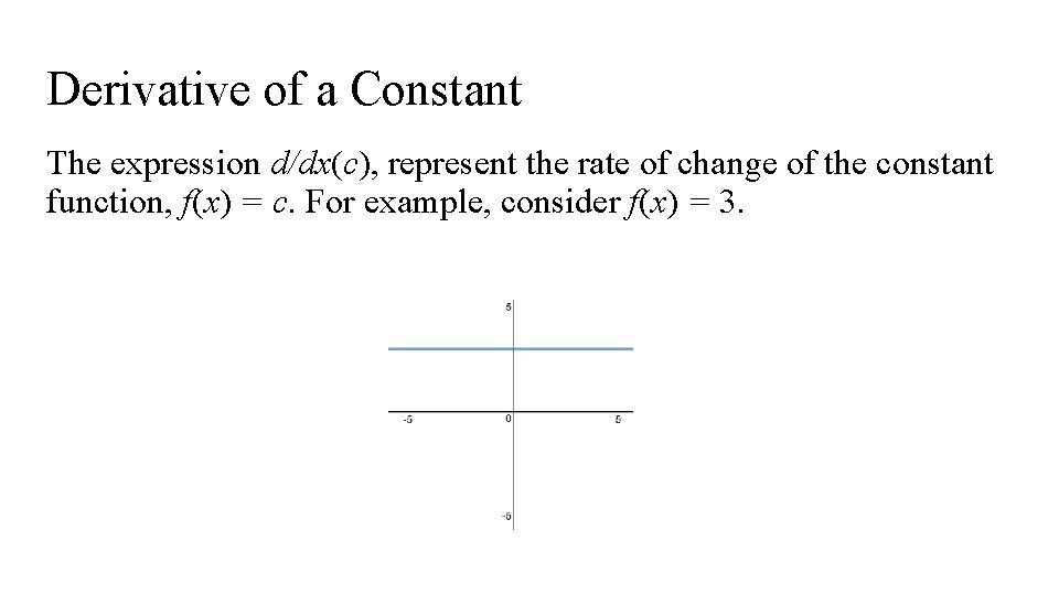
Properties of Derivatives Below are two useful properties of the derivative. 1. d/dx[f(x) + g(x)] = df/dx + dg/dx. 1. d/dx(c) = 0, where c is a constant.

Derivative of a Constant The expression d/dx(c), represent the rate of change of the constant function, f(x) = c. For example, consider f(x) = 3.

Infecteds S(t) + I(t) + R(t) = N d/dt[S(t) + I(t) + R(t)] = d/dt[N] d. S/dt + d. I/dt + d. R/dt = 0 d. I/dt = -d. S/dt - d. R/dt d. I/dt = -(-r. SI) - a. I d. I/dt = r. SI - a. I

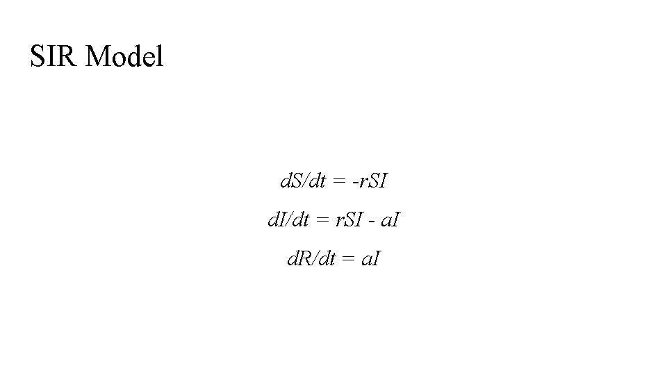
SIR Model d. S/dt = -r. SI d. I/dt = r. SI - a. I d. R/dt = a. I

Go with the Flow! Fluid Dynamics Class 4: Partial Differential Equations (Part 1)

Topics ● ● Partial derivatives 1 D laplacian 1 D finite difference method Numerical solutions to linear systems of equations

Go with the Flow! Fluid Dynamics Class 5: Partial Differential Equations (Part 2)

Topics ● ● ● 2 D Laplacian 2 D Finite difference method Numerical solutions

Go with the Flow! Fluid Dynamics Class 6: Fluid Dynamics

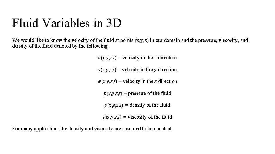
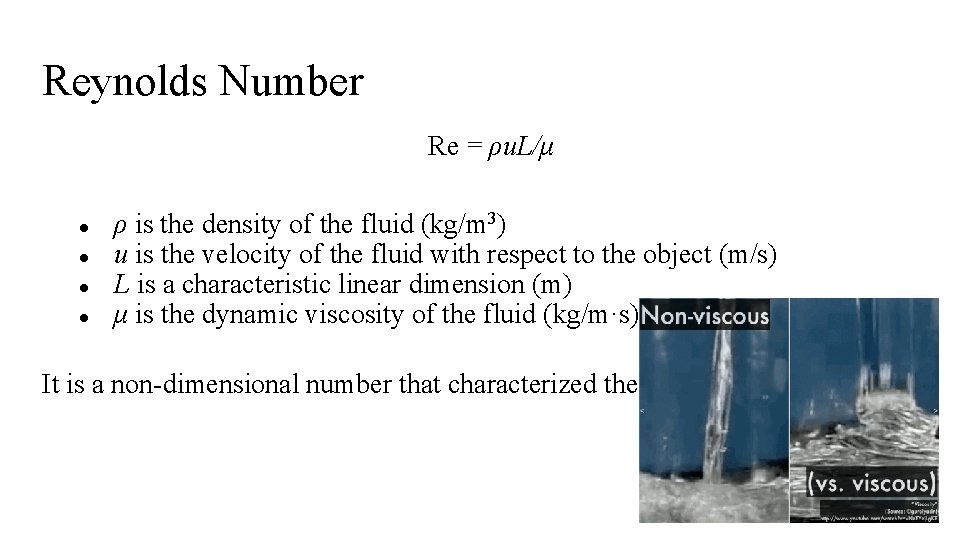
Fluid Variables in 3 D We would like to know the velocity of the fluid at points (x, y, z) in our domain and the pressure, viscosity, and density of the fluid denoted by the following. u(x, y, z, t) = velocity in the x direction v(x, y, z, t) = velocity in the y direction w(x, y, z, t) = velocity in the z direction p(x, y, z, t) = pressure of the fluid ρ(x, y, z, t) = density of the fluid μ(x, y, z, t) = viscosity of the fluid For many application, the density and viscosity are assumed to be constant.

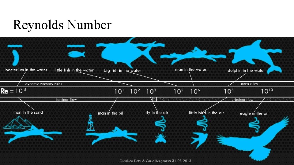
Reynolds Number Re = ρu. L/μ ● ● ρ is the density of the fluid (kg/m 3) u is the velocity of the fluid with respect to the object (m/s) L is a characteristic linear dimension (m) μ is the dynamic viscosity of the fluid (kg/m·s) It is a non-dimensional number that characterized the flow.

Reynolds Number

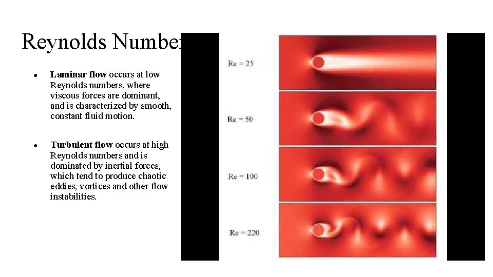
Reynolds Number ● Laminar flow occurs at low Reynolds numbers, where viscous forces are dominant, and is characterized by smooth, constant fluid motion. ● Turbulent flow occurs at high Reynolds numbers and is dominated by inertial forces, which tend to produce chaotic eddies, vortices and other flow instabilities.

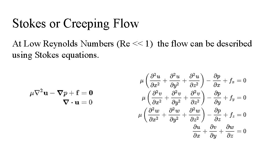
Stokes or Creeping Flow At Low Reynolds Numbers (Re << 1) the flow can be described using Stokes equations.

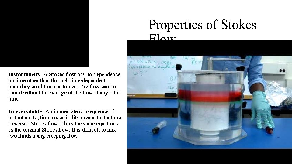
Properties of Stokes Flow Instantaneity: A Stokes flow has no dependence on time other than through time-dependent boundary conditions or forces. The flow can be found without knowledge of the flow at any other time. Irreversibility: An immediate consequence of instantaneity, time-reversibility means that a time -reversed Stokes flow solves the same equations as the original Stokes flow. It is difficult to mix two fluids using creeping flow.

Numerically Solving the Stokes Equations ● Convert the Stokes equations it into a series of Poisson problems by decoupling the velocity components and pressure. ● These can then be solved using the finite difference method discussed in class yesterday.

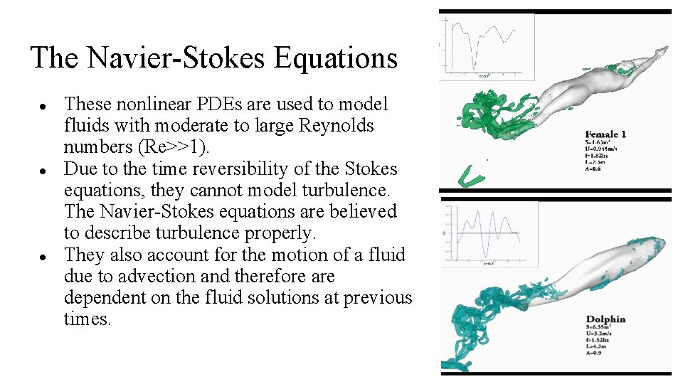
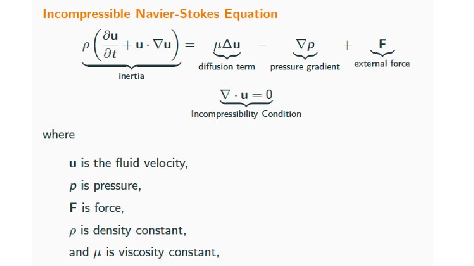
The Navier-Stokes Equations ● ● ● These nonlinear PDEs are used to model fluids with moderate to large Reynolds numbers (Re>>1). Due to the time reversibility of the Stokes equations, they cannot model turbulence. The Navier-Stokes equations are believed to describe turbulence properly. They also account for the motion of a fluid due to advection and therefore are dependent on the fluid solutions at previous times.

Why is numerical analysis so important? ● There is no proof for the questions: ○ ○ ● ● Do solutions to the Navier-Stokes equations exist? Are they unique? Clay Mathematics Institute offers a million dollar prize for proof or counter example! Analytical solutions can only be found in a few special cases. ○ ○ ○ Non-linear terms in the Navier–Stokes equations equal to zero (Poiseuille Flow, Couette Flow, Oscillatory Stokes Boundary Layer) Interesting examples (Jeffery–Hamel Flow, Von Kármán Swirling Flow, Stagnation Point Flow, Landau–Squire Jet, Taylor–Green Vortex) Note that the existence of these exact solutions does not imply they are stable: turbulence may develop at higher Reynolds numbers.

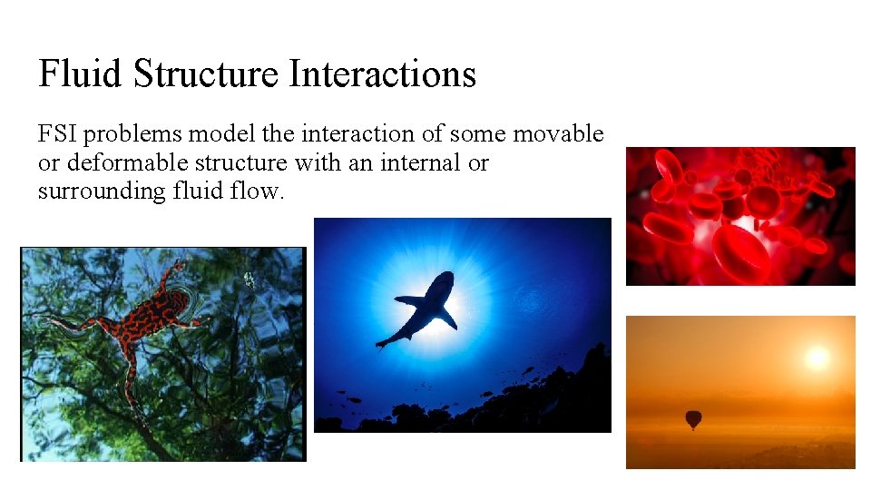
Fluid Structure Interactions FSI problems model the interaction of some movable or deformable structure with an internal or surrounding fluid flow.

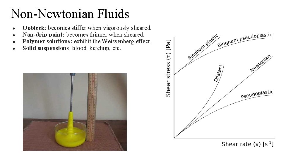
Newtonian Fluids ● Newtonian fluids are the simplest mathematical models of fluids that account for viscosity. ● While no real fluid fits the definition perfectly, many common liquids and gases, such as water and air, can be assumed to be Newtonian for practical calculations under ordinary conditions. ● In a non-Newtonian fluid, the relation between the shear stress and the shear rate is different. The fluid can even exhibit time-dependent viscosity. Therefore, a constant coefficient of viscosity cannot be defined.

Non-Newtonian Fluids ● ● Oobleck: becomes stiffer when vigorously sheared. Non-drip paint: becomes thinner when sheared. Polymer solutions: exhibit the Weissenberg effect. Solid suspensions: blood, ketchup, etc.