MECE 5005 Fluid Power Dynamics L 5 cr

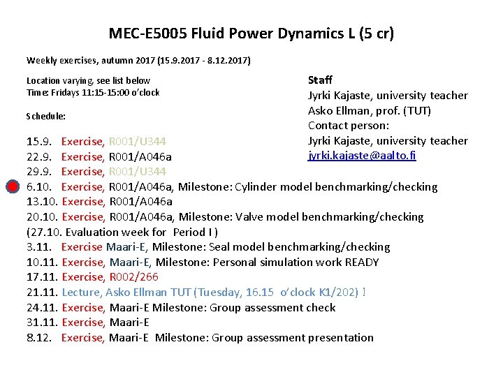
MEC-E 5005 Fluid Power Dynamics L (5 cr) Weekly exercises, autumn 2017 (15. 9. 2017 - 8. 12. 2017) Location varying, see list below Time: Fridays 11: 15 -15: 00 o’clock Schedule: Staff Jyrki Kajaste, university teacher Asko Ellman, prof. (TUT) Contact person: Jyrki Kajaste, university teacher jyrki. kajaste@aalto. fi 15. 9. Exercise, R 001/U 344 22. 9. Exercise, R 001/A 046 a 29. 9. Exercise, R 001/U 344 6. 10. Exercise, R 001/A 046 a, Milestone: Cylinder model benchmarking/checking 13. 10. Exercise, R 001/A 046 a 20. 10. Exercise, R 001/A 046 a, Milestone: Valve model benchmarking/checking (27. 10. Evaluation week for Period I ) 3. 11. Exercise Maari-E, Milestone: Seal model benchmarking/checking 10. 11. Exercise, Maari-E, Milestone: Personal simulation work READY 17. 11. Exercise, R 002/266 21. 11. Lecture, Asko Ellman TUT (Tuesday, 16. 15 o’clock K 1/202) ! 24. 11. Exercise, Maari-E Milestone: Group assessment check 31. 11. Exercise, Maari-E 8. 12. Exercise, Maari-E Milestone: Group assessment presentation

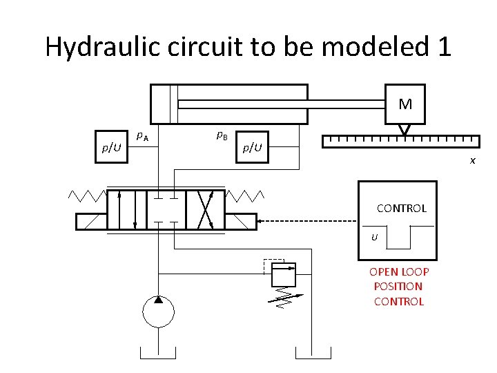
Hydraulic circuit to be modeled 1 M p/U p. A p. B p/U x CONTROL U OPEN LOOP POSITION CONTROL

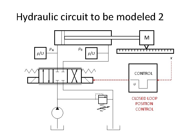
Hydraulic circuit to be modeled 2 M p/U p. A p. B p/U x CONTROL U CLOSED LOOP POSITION CONTROL

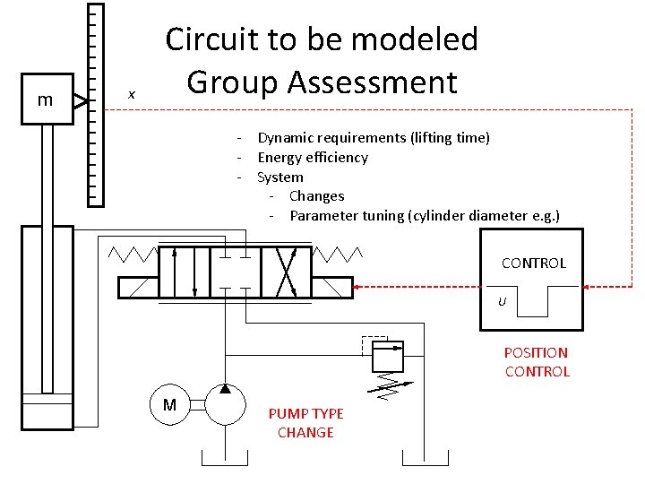
m x Circuit to be modeled Group Assessment - Dynamic requirements (lifting time) - Energy efficiency - System - Changes - Parameter tuning (cylinder diameter e. g. ) CONTROL U POSITION CONTROL M PUMP TYPE CHANGE

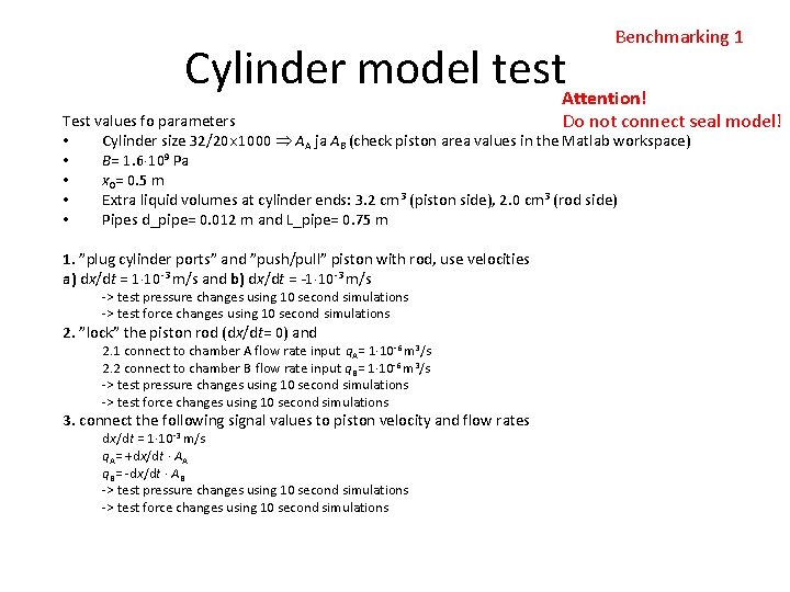
Benchmarking 1 Cylinder model test. Attention! Test values fo parameters Do not connect seal model! • Cylinder size 32/20 1000 AA ja AB (check piston area values in the Matlab workspace) • B= 1. 6 109 Pa • x 0= 0. 5 m • Extra liquid volumes at cylinder ends: 3. 2 cm 3 (piston side), 2. 0 cm 3 (rod side) • Pipes d_pipe= 0. 012 m and L_pipe= 0. 75 m 1. ”plug cylinder ports” and ”push/pull” piston with rod, use velocities a) dx/dt = 1 10 -3 m/s and b) dx/dt = -1 10 -3 m/s -> test pressure changes using 10 second simulations -> test force changes using 10 second simulations 2. ”lock” the piston rod (dx/dt= 0) and 2. 1 connect to chamber A flow rate input q. A= 1 10 -6 m 3/s 2. 2 connect to chamber B flow rate input q. B= 1 10 -6 m 3/s -> test pressure changes using 10 second simulations -> test force changes using 10 second simulations 3. connect the following signal values to piston velocity and flow rates dx/dt = 1 10 -3 m/s q. A= +dx/dt AA q. B= -dx/dt AB -> test pressure changes using 10 second simulations -> test force changes using 10 second simulations

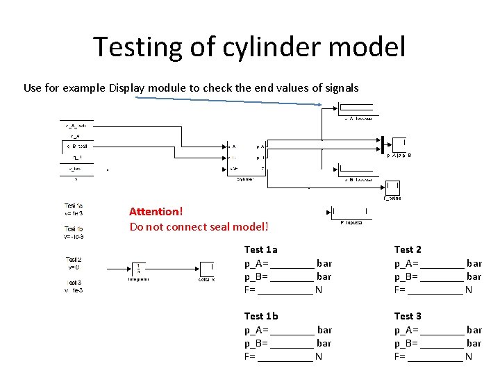
Testing of cylinder model Use for example Display module to check the end values of signals Attention! Do not connect seal model! Test 1 a p_A= ____ bar p_B= ____ bar F= _____ N Test 2 p_A= ____ bar p_B= ____ bar F= _____ N Test 1 b p_A= ____ bar p_B= ____ bar F= _____ N Test 3 p_A= ____ bar p_B= ____ bar F= _____ N

Cylinder model benchmarking/checking Documenting • Use blank Word document (or another word processor) • Models to be documented (copying: Edit Copy Model To Clipboard) – Chamber A – Chamber B – Cylinder model ( Force) • Test results: – End values after 10 second simulation time (p. A, p. B, F) • This document material is usable in your personal simulation model report!

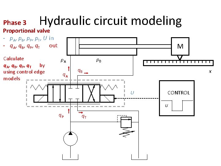
Phase 3 Hydraulic circuit modeling Proportional valve - p. A, p. B, p. P, p. T, U in - q. A, q. B, q. P, q. T out Calculate q. A, q. B, q. P, q. T by using control edge models M p. B p. A q. B x U CONTROL U q. P q. T

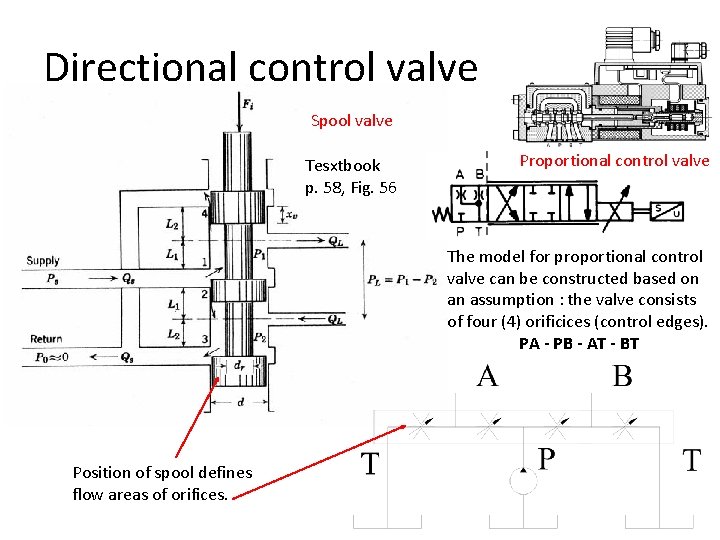
Directional control valve Spool valve Tesxtbook p. 58, Fig. 56 Proportional control valve The model for proportional control valve can be constructed based on an assumption : the valve consists of four (4) orificices (control edges). PA - PB - AT - BT Position of spool defines flow areas of orifices.

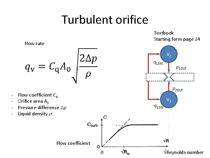
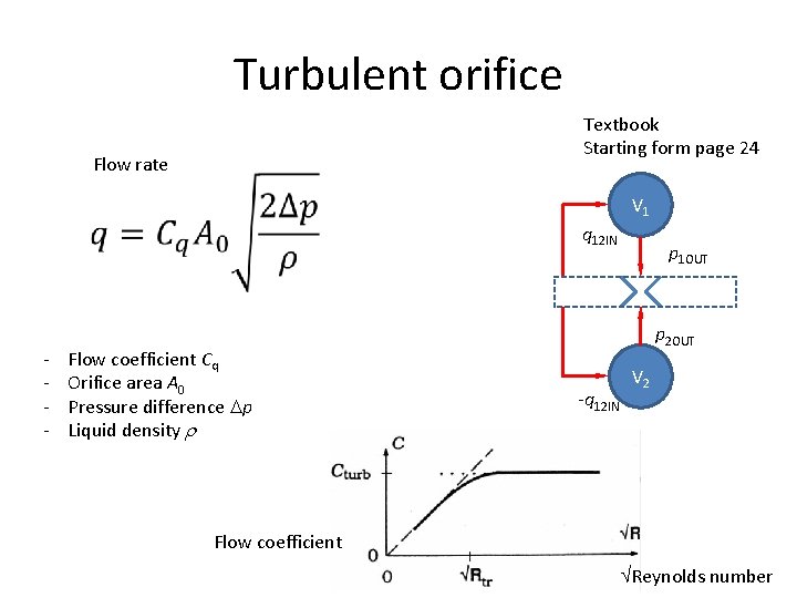
Turbulent orifice Textbook Starting form page 24 Flow rate V 1 q 12 IN - Flow coefficient Cq Orifice area A 0 Pressure difference p Liquid density p 1 OUT p 2 OUT -q 12 IN V 2 Flow coefficient Reynolds number

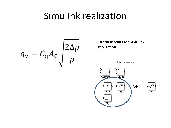
Simulink realization Useful moduls for Simulink realization OR

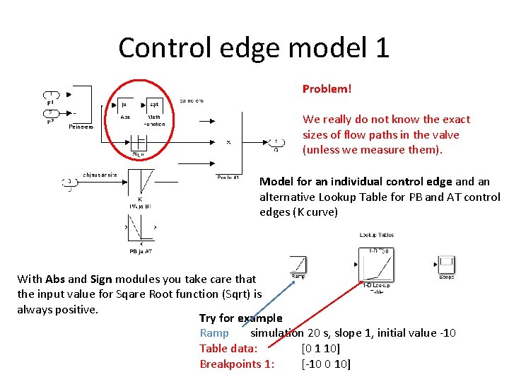
Control edge model 1 Problem! We really do not know the exact sizes of flow paths in the valve (unless we measure them). Model for an individual control edge and an alternative Lookup Table for PB and AT control edges (K curve) With Abs and Sign modules you take care that the input value for Sqare Root function (Sqrt) is always positive. Try for example Ramp simulation 20 s, slope 1, initial value -10 Table data: [0 1 10] Breakpoints 1: [-10 0 10]

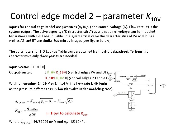
Control edge model 2 – parameter K 10 V Inputs for control edge model are pressures (p 1 ja p 1) and control voltage (U). Flow rate (q) is the system output. The valve capacity (”K characteristics”) as a function of voltage can be modeled for instance with 1 -D Lookup Table. In a symmetrical valve the characteristics of PA and PB as well as AT and BT are similar but mirros images (see figure below). The parameters for 1 -D Lookup Table can be obtained from valve’s datasheet. To form the characteristics only three points are needed. Input-vector: [-10 0 10] Output-vector: [0 K_0 V K_10 V] (control edges PA and BT). [K_10 V K_0 V 0] (control edges PB and AT) With full opening (U= 10 V or U= -10 V) the flow rate is 40 l/min as the pressure difference is 35 bar (for valve in the modeling case). How to calculate K 10 V Where qv orifice= 40/60000 m 3/s and p= 35 105 Pa.

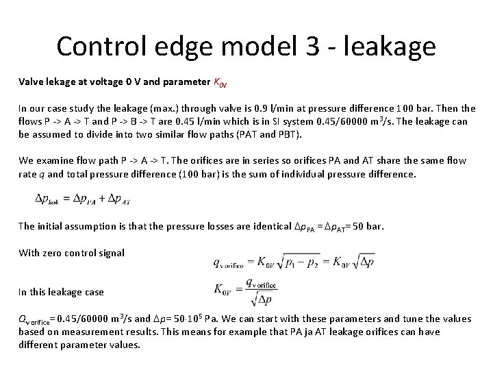
Control edge model 3 - leakage Valve lekage at voltage 0 V and parameter K 0 V In our case study the leakage (max. ) through valve is 0. 9 l/min at pressure difference 100 bar. Then the flows P -> A -> T and P -> B -> T are 0. 45 l/min which is in SI system 0. 45/60000 m 3/s. The leakage can be assumed to divide into two similar flow paths (PAT and PBT). We examine flow path P -> A -> T. The orifices are in series so orifices PA and AT share the same flow rate q and total pressure difference (100 bar) is the sum of individual pressure difference. The initial assumption is that the pressure losses are identical p. PA = p. AT= 50 bar. With zero control signal In this leakage case Qv orifice= 0. 45/60000 m 3/s and p= 50 105 Pa. We can start with these parameters and tune the values based on measurement results. This means for example that PA ja AT leakage orifices can have different parameter values.

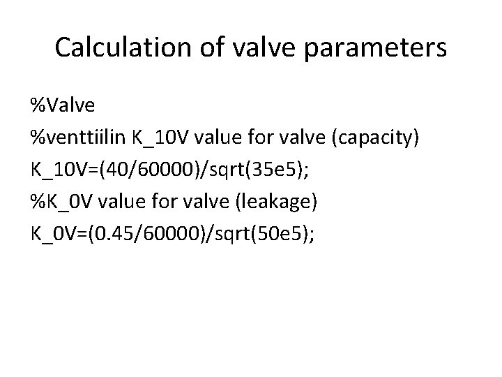
K values for orifices from valve data sheet K_10 V=(40/60000)/sqrt(35 e 5); %full opening (10 V) K_0 V=(0. 45/60000)/sqrt(50 e 5); %leakage at ”closed”position (0 V) About the leakage It can be assumed that all of the four orifices are similar as the valve is in central (”closed”) position. However the valve is of spool type and there is some leakage. All orifices (K_0 V): 0. 45 l/min @ 50 bar Actuator channels A and B blocked, no flow. 0. 45 l/min 0 bar 0. 9 l/min 100 bar Spool at center position: from the data sheet • Pump pressure 100 bar • Total flow below 0. 9 l/min

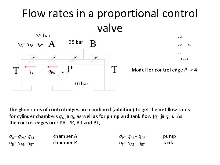
Flow rates in a proportional control valve 35 bar q. A= q. PA- q. AT Model for control edge P -> A q. PA 70 bar The glow rates of control edges are combined (addition) to get the net flow rates for cylinder chambers q. A ja q. B as well as for pump and tank flow (q. P ja q. T ). As the control edges are: PA, PB, AT and BT, q. A= q. PA- q. AT chamber A q. P= q. PA+ q. PB pump q. B= q. PB- q. BT chamber B q. T= q. AT+ q. BT tank

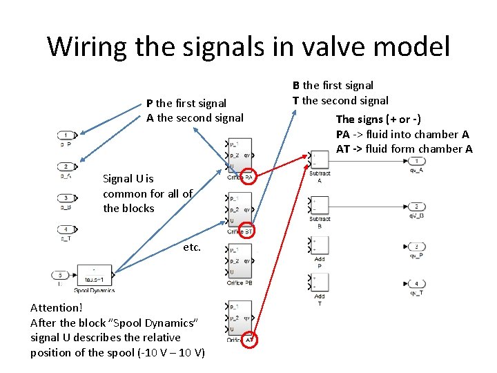
Wiring the signals in valve model P the first signal A the second signal Signal U is common for all of the blocks etc. Attention! After the block ”Spool Dynamics” signal U describes the relative position of the spool (-10 V – 10 V) B the first signal T the second signal The signs (+ or -) PA -> fluid into chamber A AT -> fluid form chamber A

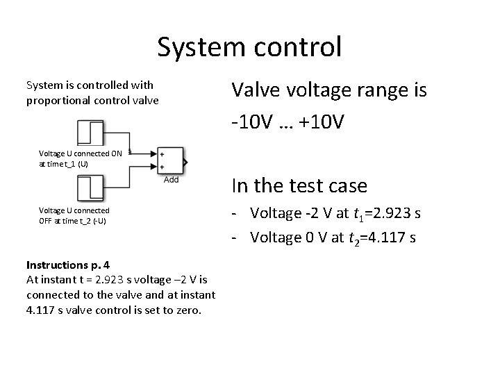
System control System is controlled with proportional control valve Valve voltage range is -10 V … +10 V Voltage U connected ON at time t_1 (U) In the test case Voltage U connected OFF at time t_2 (-U) Instructions p. 4 At instant t = 2. 923 s voltage – 2 V is connected to the valve and at instant 4. 117 s valve control is set to zero. - Voltage -2 V at t 1=2. 923 s - Voltage 0 V at t 2=4. 117 s

Calculation of valve parameters %Valve %venttiilin K_10 V value for valve (capacity) K_10 V=(40/60000)/sqrt(35 e 5); %K_0 V value for valve (leakage) K_0 V=(0. 45/60000)/sqrt(50 e 5);

Turbulent orifice Textbook Starting form page 24 Flow rate V 1 q 12 IN - Flow coefficient Cq Orifice area A 0 Pressure difference p Liquid density p 1 OUT p 2 OUT -q 12 IN V 2 Flow coefficient Reynolds number

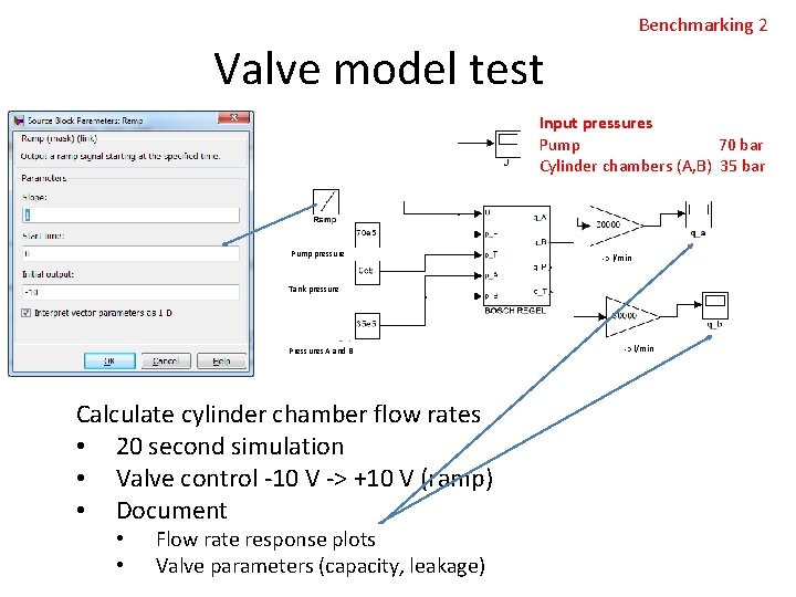
Benchmarking 2 Proportional control valve model • Use blank Word document (or another word processor) • Models to be documented (copying: Edit Copy Model To Clipboard) – Orifice model PA (BT) – Orifice model PB (AT) – Overall valve model ( A and B chamber flow rates) • Include parameter values and test results: – Valve parameters K_10 V and K_0 V (full capacity and leakage) – Flow rate response (q. A, q. B) plot, with control -10 V -> +10 V (ramp) • This document material is usable in your personal simulation model report!

Benchmarking 2 Valve model test Input pressures Pump 70 bar Cylinder chambers (A, B) 35 bar Pump pressure Tank pressure Pressures A and B Calculate cylinder chamber flow rates • 20 second simulation • Valve control -10 V -> +10 V (ramp) • Document • • -> l/min Flow rate response plots Valve parameters (capacity, leakage) -> l/min

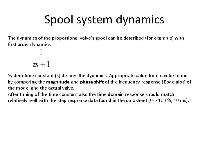
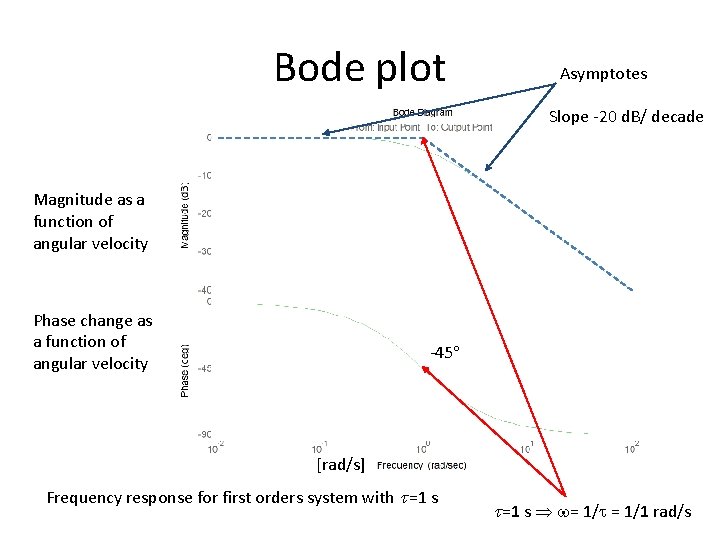
Spool system dynamics The dynamics of the proportional valve’s spool can be described (for example) with first order dynamics. System time constant ( ) defines the dynamics. Appropriate value for it can be found by comparing the magnitude and phase shift of the frequency response (Bode plot) of the model and the actual valve. After tuning of the time constant also the time domain response should match relatively well with the step response data found in the datasheet (0 -> 100 %, 10 ms).

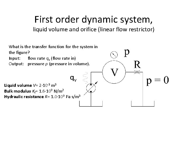
First order dynamic system, liquid volume and orifice (linear flow restrictor) What is the transfer function for the system in the figure? Input: flow rate qv (flow rate in) Output: pressure p (pressure in volume). qv Liquid volume V= 2 10 -3 m 3 Bulk modulus Kf= 1. 6 109 N/m 2 Hydraulic resistance R= 1. 0 109 Pa s/m 3

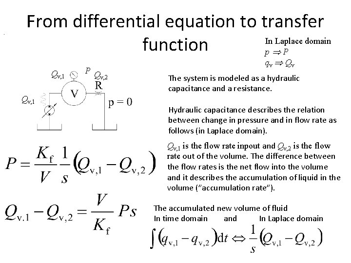
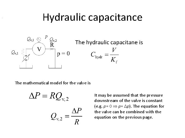
. From differential equation to transfer In Laplace domain function p P Qv, 1 P Q v, 2 qv Qv The system is modeled as a hydraulic capacitance and a resistance. Hydraulic capacitance describes the relation between change in pressure and in flow rate as follows (in Laplace domain). Qv, 1 is the flow rate inpout and Qv, 2 is the flow rate out of the volume. The difference between the flow rates is the net flow into the volume and it describes the accumulation of liquid in the volume (”accumulation rate”). The accumulated new volume of fluid In time domain and In Laplace domain

Hydraulic capacitance . Qv, 1 P Q v, 2 The hydraulic capacitane is Qv, 1 The mathematical model for the valve is It may be assumed that the pressure downstream of the valve is constant (e. g. p= 0 p= p). The equation for the valve can be combined with the equation on the previous page.

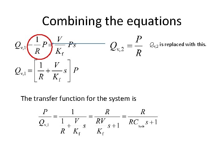
Combining the equations Qv, 2 is replaced with this. The transfer function for the system is

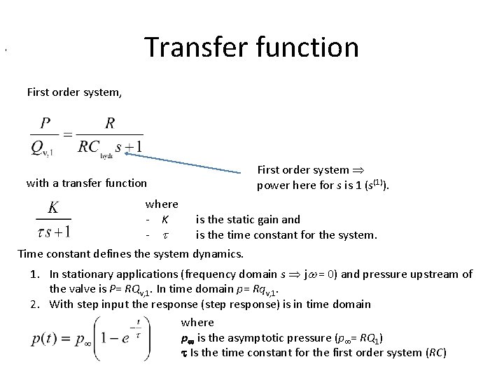
Transfer function , First order system power here for s is 1 (s(1)). with a transfer function where - K - is the static gain and is the time constant for the system. Time constant defines the system dynamics. 1. In stationary applications (frequency domain s j = 0) and pressure upstream of the valve is P= RQv, 1. In time domain p= Rqv, 1. 2. With step input the response (step response) is in time domain where p is the asymptotic pressure (p = RQ 1) Is the time constant for the first order system (RC)

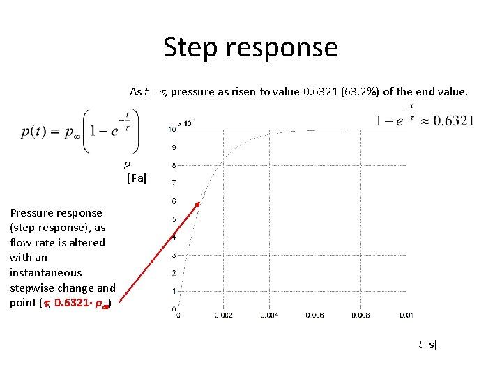
Step response As t = , pressure as risen to value 0. 6321 (63. 2%) of the end value. p [Pa] Pressure response (step response), as flow rate is altered with an instantaneous stepwise change and point ( , 0. 6321 p ) t [s]

Bode plot Asymptotes Slope -20 d. B/ decade Magnitude as a function of angular velocity Phase change as a function of angular velocity -45 [rad/s] Frequency response for first orders system with =1 s = 1/1 rad/s

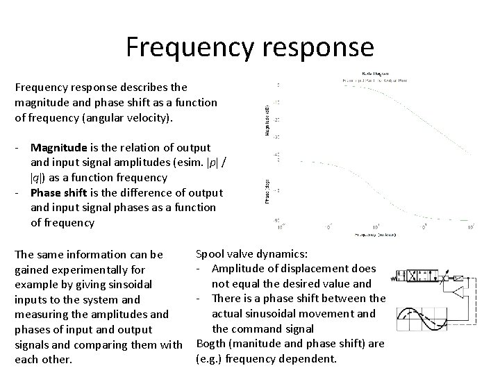
Frequency response describes the magnitude and phase shift as a function of frequency (angular velocity). - Magnitude is the relation of output and input signal amplitudes (esim. p / q ) as a function frequency - Phase shift is the difference of output and input signal phases as a function of frequency The same information can be gained experimentally for example by giving sinsoidal inputs to the system and measuring the amplitudes and phases of input and output signals and comparing them with each other. Spool valve dynamics: - Amplitude of displacement does not equal the desired value and - There is a phase shift between the actual sinusoidal movement and the command signal Bogth (manitude and phase shift) are (e. g. ) frequency dependent.

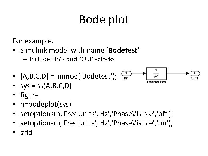
Bode plot For example. • Simulink model with name ’Bodetest’ – Include ”In”- and ”Out”-blocks • • [A, B, C, D] = linmod('Bodetest'); sys = ss(A, B, C, D) figure h=bodeplot(sys) setoptions(h, 'Freq. Units', 'Hz', 'Phase. Visible', 'off'); setoptions(h, 'Freq. Units', 'Hz', 'Phase. Visible', 'on'); grid

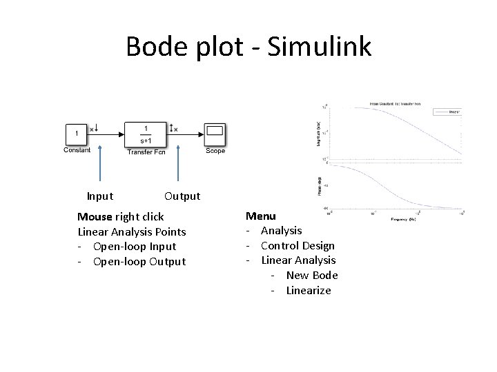
Bode plot - Simulink Input Output Mouse right click Linear Analysis Points - Open-loop Input - Open-loop Output Menu - Analysis - Control Design - Linear Analysis - New Bode - Linearize

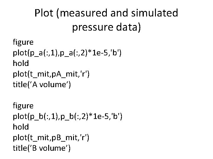
Plot (measured and simulated pressure data) figure plot(p_a(: , 1), p_a(: , 2)*1 e-5, 'b') hold plot(t_mit, p. A_mit, 'r') title(’A volume’) figure plot(p_b(: , 1), p_b(: , 2)*1 e-5, 'b') hold plot(t_mit, p. B_mit, 'r') title(’B volume’)