Econometrics Lecture 3 Regression Models Interpretation and Comparison

Econometrics - Lecture 3 Regression Models: Interpretation and Comparison

Contents n The Linear Model: Interpretation Selection of Regressors n Specification of the Functional Form n Oct 30, 2015 Hackl, Econometrics, Lecture 3 2

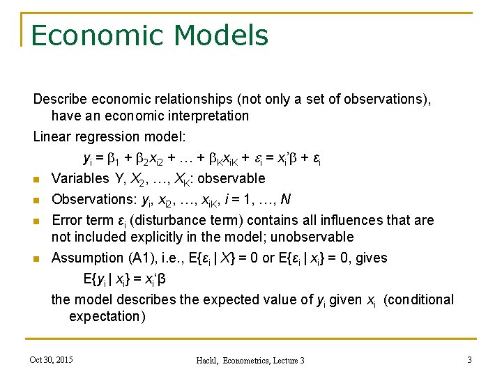
Economic Models Describe economic relationships (not only a set of observations), have an economic interpretation Linear regression model: yi = 1 + 2 xi 2 + … + Kxi. K + ei = xi’ + εi n Variables Y, X 2, …, XK: observable n Observations: yi, xi 2, …, xi. K, i = 1, …, N n Error term εi (disturbance term) contains all influences that are not included explicitly in the model; unobservable n Assumption (A 1), i. e. , E{εi | X} = 0 or E{εi | xi} = 0, gives E{yi | xi} = xi‘β the model describes the expected value of yi given xi (conditional expectation) Oct 30, 2015 Hackl, Econometrics, Lecture 3 3

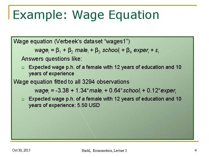
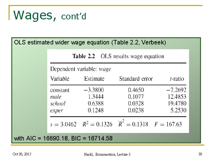
Example: Wage Equation Wage equation (Verbeek’s dataset “wages 1”) wagei = β 1 + β 2 malei + β 3 schooli + β 4 experi + εi Answers questions like: q Expected wage p. h. of a female with 12 years of education and 10 years of experience Wage equation fitted to all 3294 observations wagei = -3. 38 + 1. 34*malei + 0. 64*schooli + 0. 12*experi q Expected wage p. h. of a female with 12 years of education and 10 years of experience: 5. 50 USD Oct 30, 2015 Hackl, Econometrics, Lecture 3 4

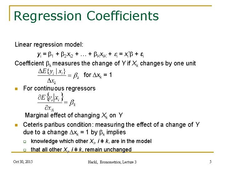
Regression Coefficients Linear regression model: yi = 1 + 2 xi 2 + … + Kxi. K + ei = xi’ + εi Coefficient k measures the change of Y if Xk changes by one unit for ∆xk = 1 n For continuous regressors n Marginal effect of changing Xk on Y Ceteris paribus condition: measuring the effect of a change of Y due to a change ∆xk = 1 by k implies q knowledge which other Xi, i ǂ k, are in the model q that all other Xi, i ǂ k, remain unchanged Oct 30, 2015 Hackl, Econometrics, Lecture 3 5

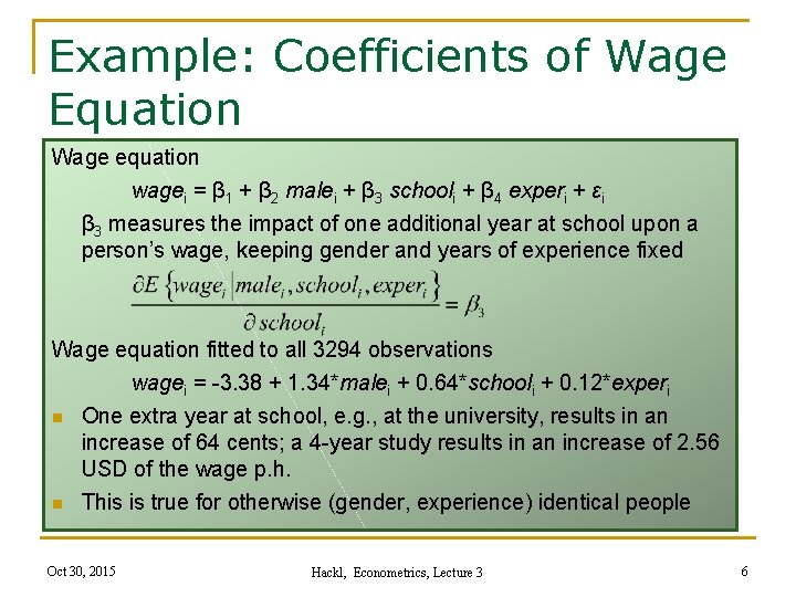
Example: Coefficients of Wage Equation Wage equation wagei = β 1 + β 2 malei + β 3 schooli + β 4 experi + εi β 3 measures the impact of one additional year at school upon a person’s wage, keeping gender and years of experience fixed Wage equation fitted to all 3294 observations wagei = -3. 38 + 1. 34*malei + 0. 64*schooli + 0. 12*experi n One extra year at school, e. g. , at the university, results in an increase of 64 cents; a 4 -year study results in an increase of 2. 56 USD of the wage p. h. n This is true for otherwise (gender, experience) identical people Oct 30, 2015 Hackl, Econometrics, Lecture 3 6

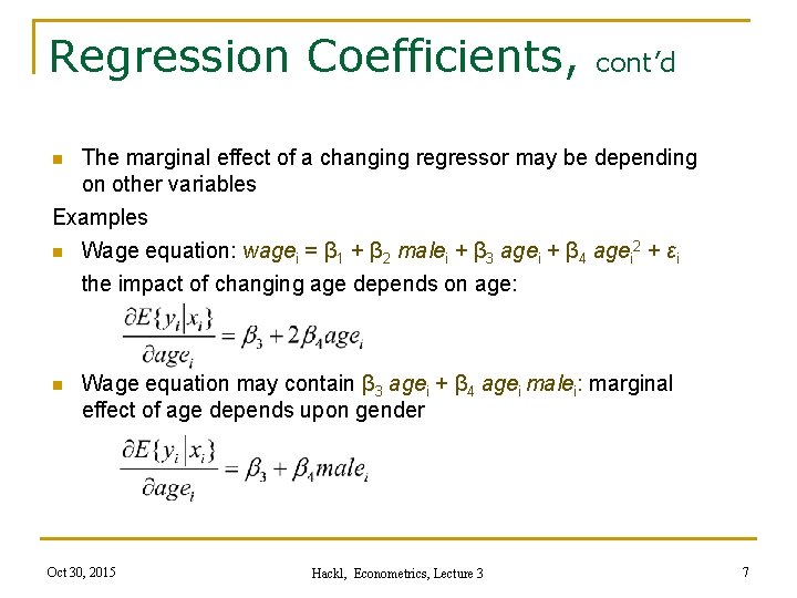
Regression Coefficients, n cont’d The marginal effect of a changing regressor may be depending on other variables Examples n Wage equation: wagei = β 1 + β 2 malei + β 3 agei + β 4 agei 2 + εi the impact of changing age depends on age: n Wage equation may contain β 3 agei + β 4 agei malei: marginal effect of age depends upon gender Oct 30, 2015 Hackl, Econometrics, Lecture 3 7

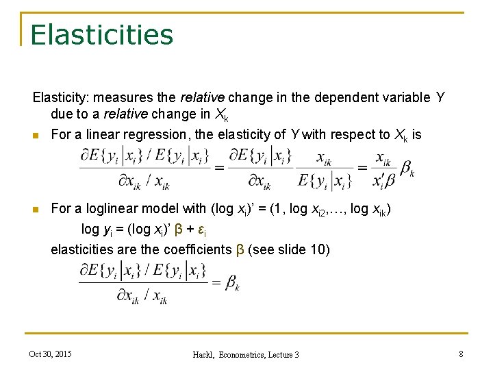
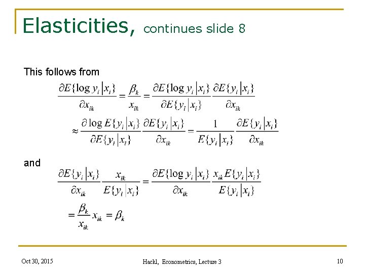
Elasticities Elasticity: measures the relative change in the dependent variable Y due to a relative change in Xk n For a linear regression, the elasticity of Y with respect to Xk is n For a loglinear model with (log xi)’ = (1, log xi 2, …, log xik) log yi = (log xi)’ β + εi elasticities are the coefficients β (see slide 10) Oct 30, 2015 Hackl, Econometrics, Lecture 3 8

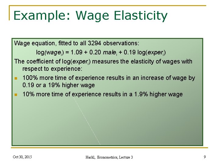
Example: Wage Elasticity Wage equation, fitted to all 3294 observations: log(wagei) = 1. 09 + 0. 20 malei + 0. 19 log(experi) The coefficient of log(experi) measures the elasticity of wages with respect to experience: n 100% more time of experience results in an increase of wage by 0. 19 or a 19% higher wage n 10% more time of experience results in a 1. 9% higher wage Oct 30, 2015 Hackl, Econometrics, Lecture 3 9

Elasticities, continues slide 8 This follows from and Oct 30, 2015 Hackl, Econometrics, Lecture 3 10

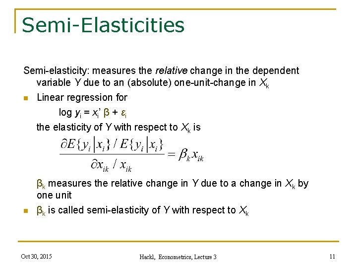
Semi-Elasticities Semi-elasticity: measures the relative change in the dependent variable Y due to an (absolute) one-unit-change in Xk n n Linear regression for log yi = xi’ β + εi the elasticity of Y with respect to Xk is βk measures the relative change in Y due to a change in Xk by one unit βk is called semi-elasticity of Y with respect to Xk Oct 30, 2015 Hackl, Econometrics, Lecture 3 11

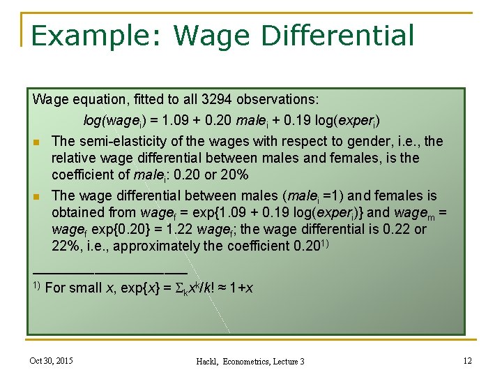
Example: Wage Differential Wage equation, fitted to all 3294 observations: log(wagei) = 1. 09 + 0. 20 malei + 0. 19 log(experi) n n The semi-elasticity of the wages with respect to gender, i. e. , the relative wage differential between males and females, is the coefficient of malei: 0. 20 or 20% The wage differential between males (malei =1) and females is obtained from wagef = exp{1. 09 + 0. 19 log(experi)} and wagem = wagef exp{0. 20} = 1. 22 wagef; the wage differential is 0. 22 or 22%, i. e. , approximately the coefficient 0. 201) __________ 1) For small x, exp{x} = S xk/k! ≈ 1+x k Oct 30, 2015 Hackl, Econometrics, Lecture 3 12

Contents n The Linear Model: Interpretation Selection of Regressors n Specification of the Functional Form n Oct 30, 2015 Hackl, Econometrics, Lecture 3 13

Selection of Regressors Specification errors: n Omission of a relevant variable Inclusion of an irrelevant variable Questions: n What are the consequences of a specification error? n How to avoid specification errors? n How to detect an erroneous specification? n Oct 30, 2015 Hackl, Econometrics, Lecture 3 14

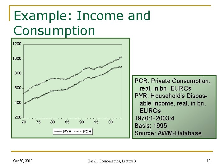
Example: Income and Consumption PCR: Private Consumption, real, in bn. EUROs PYR: Household's Disposable Income, real, in bn. EUROs 1970: 1 -2003: 4 Basis: 1995 Source: AWM-Database Oct 30, 2015 Hackl, Econometrics, Lecture 3 15

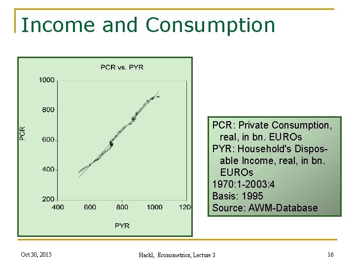
Income and Consumption PCR: Private Consumption, real, in bn. EUROs PYR: Household's Disposable Income, real, in bn. EUROs 1970: 1 -2003: 4 Basis: 1995 Source: AWM-Database Oct 30, 2015 Hackl, Econometrics, Lecture 3 16

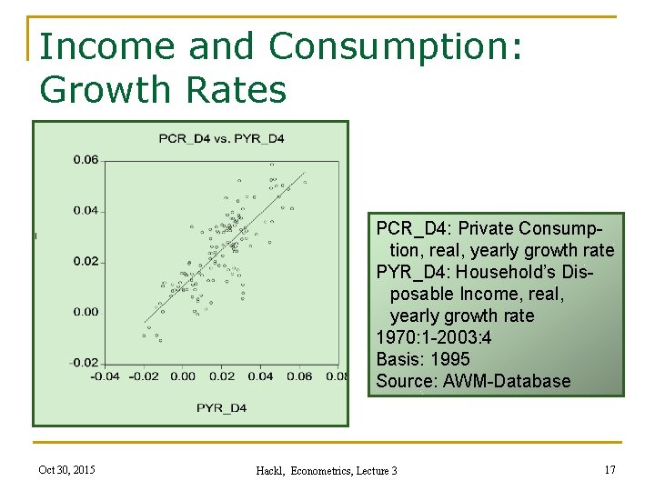
Income and Consumption: Growth Rates PCR_D 4: Private Consumption, real, yearly growth rate PYR_D 4: Household’s Disposable Income, real, yearly growth rate 1970: 1 -2003: 4 Basis: 1995 Source: AWM-Database Oct 30, 2015 Hackl, Econometrics, Lecture 3 17

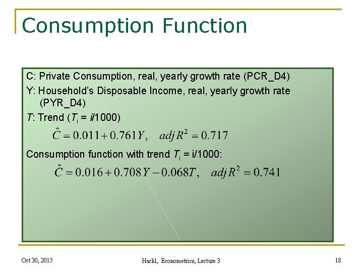
Consumption Function C: Private Consumption, real, yearly growth rate (PCR_D 4) Y: Household’s Disposable Income, real, yearly growth rate (PYR_D 4) T: Trend (Ti = i/1000) Consumption function with trend Ti = i/1000: Oct 30, 2015 Hackl, Econometrics, Lecture 3 18

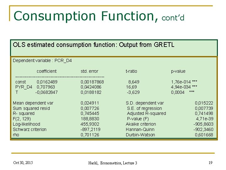
Consumption Function, cont’d OLS estimated consumption function: Output from GRETL Dependent variable : PCR_D 4 coefficient std. error ------------------------------const 0, 0162489 0, 00187868 PYR_D 4 0, 707963 0, 0424086 T -0, 0682847 0, 0188182 Mean dependent var Sum squared resid R- squared F(2, 129) Log-likelihood Schwarz criterion rho Oct 30, 2015 0, 024911 0, 007726 0, 745445 188, 8830 455, 9302 -897, 2119 0, 701126 t-ratio p-value 8, 649 16, 69 -3, 629 1, 76 e-014 *** 4, 94 e-034 *** 0, 0004 *** S. D. dependent var S. E. of regression Adjusted R-squared P-value (F) Akaike criterion Hannan-Quinn Durbin-Watson Hackl, Econometrics, Lecture 3 0, 015222 0, 007739 0, 741498 4, 71 e-39 -905, 8603 -902, 3460 0, 601668 19

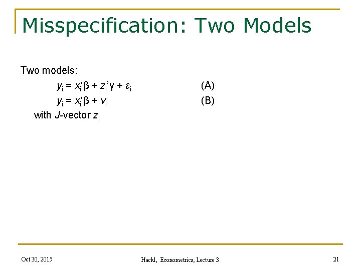
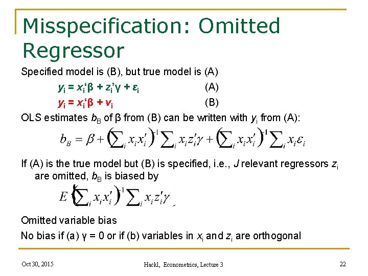
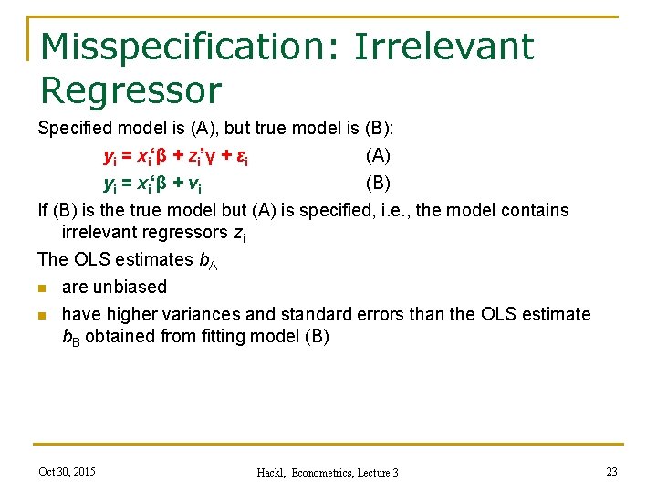
Consequences of specification errors: n Omission of a relevant variable n Inclusion of a irrelevant variable Oct 30, 2015 Hackl, Econometrics, Lecture 3 20

Misspecification: Two Models Two models: yi = xi‘β + zi’γ + εi yi = xi‘β + vi with J-vector zi Oct 30, 2015 (A) (B) Hackl, Econometrics, Lecture 3 21

Misspecification: Omitted Regressor Specified model is (B), but true model is (A) yi = xi‘β + zi’γ + εi (A) yi = xi‘β + vi (B) OLS estimates b. B of β from (B) can be written with yi from (A): If (A) is the true model but (B) is specified, i. e. , J relevant regressors zi are omitted, b. B is biased by Omitted variable bias No bias if (a) γ = 0 or if (b) variables in xi and zi are orthogonal Oct 30, 2015 Hackl, Econometrics, Lecture 3 22

Misspecification: Irrelevant Regressor Specified model is (A), but true model is (B): yi = xi‘β + zi’γ + εi (A) yi = xi‘β + vi (B) If (B) is the true model but (A) is specified, i. e. , the model contains irrelevant regressors zi The OLS estimates b. A n are unbiased n have higher variances and standard errors than the OLS estimate b. B obtained from fitting model (B) Oct 30, 2015 Hackl, Econometrics, Lecture 3 23

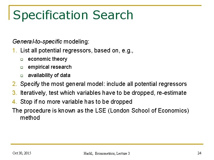
Specification Search General-to-specific modeling: 1. List all potential regressors, based on, e. g. , q economic theory q empirical research q availability of data 2. Specify the most general model: include all potential regressors 3. Iteratively, test which variables have to be dropped, re-estimate 4. Stop if no more variable has to be dropped The procedure is known as the LSE (London School of Economics) method Oct 30, 2015 Hackl, Econometrics, Lecture 3 24

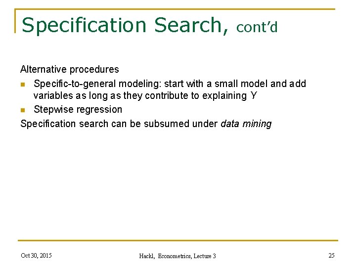
Specification Search, cont’d Alternative procedures n Specific-to-general modeling: start with a small model and add variables as long as they contribute to explaining Y n Stepwise regression Specification search can be subsumed under data mining Oct 30, 2015 Hackl, Econometrics, Lecture 3 25

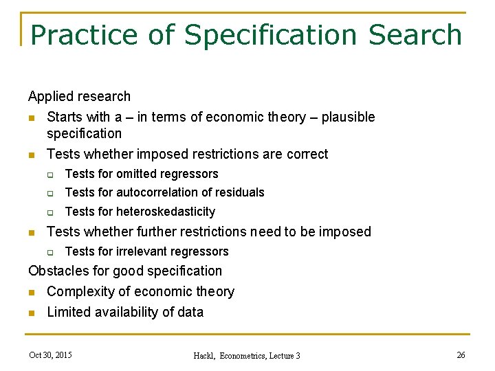
Practice of Specification Search Applied research n Starts with a – in terms of economic theory – plausible specification n Tests whether imposed restrictions are correct n q Tests for omitted regressors q Tests for autocorrelation of residuals q Tests for heteroskedasticity Tests whether further restrictions need to be imposed q Tests for irrelevant regressors Obstacles for good specification n Complexity of economic theory n Limited availability of data Oct 30, 2015 Hackl, Econometrics, Lecture 3 26

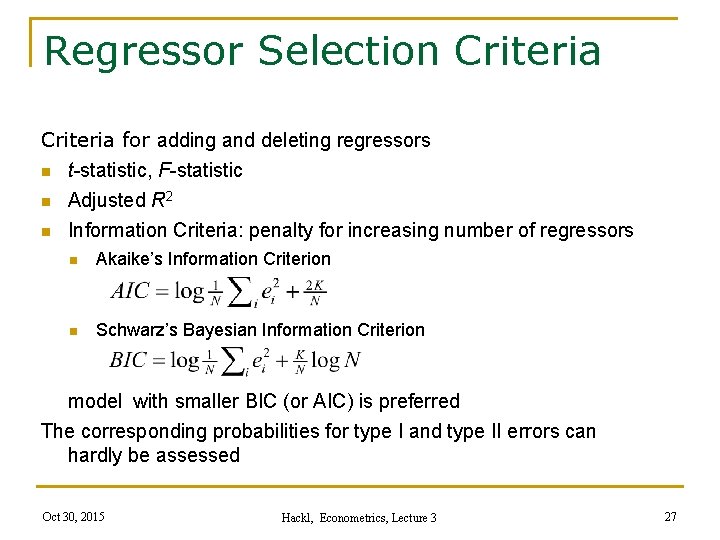
Regressor Selection Criteria for adding and deleting regressors n t-statistic, F-statistic n n Adjusted R 2 Information Criteria: penalty for increasing number of regressors n Akaike’s Information Criterion n Schwarz’s Bayesian Information Criterion model with smaller BIC (or AIC) is preferred The corresponding probabilities for type I and type II errors can hardly be assessed Oct 30, 2015 Hackl, Econometrics, Lecture 3 27

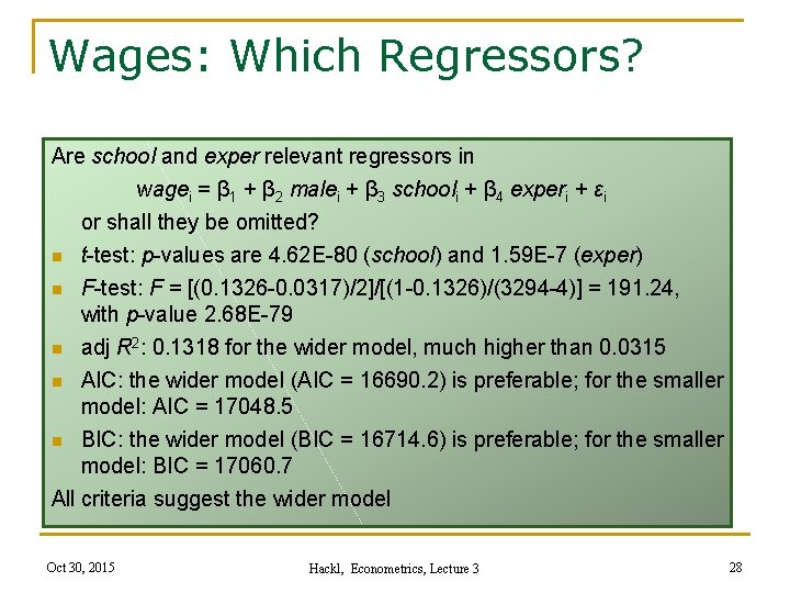
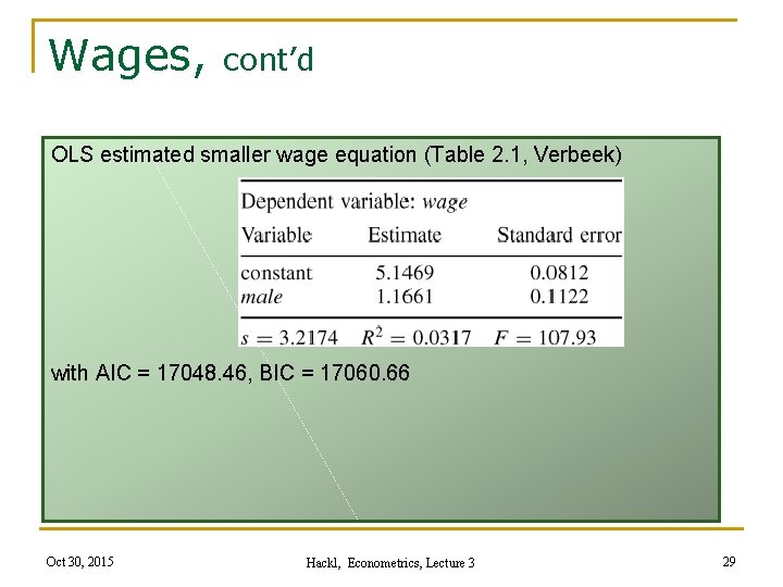
Wages: Which Regressors? Are school and exper relevant regressors in wagei = β 1 + β 2 malei + β 3 schooli + β 4 experi + εi or shall they be omitted? n t-test: p-values are 4. 62 E-80 (school) and 1. 59 E-7 (exper) n F-test: F = [(0. 1326 -0. 0317)/2]/[(1 -0. 1326)/(3294 -4)] = 191. 24, with p-value 2. 68 E-79 n adj R 2: 0. 1318 for the wider model, much higher than 0. 0315 n AIC: the wider model (AIC = 16690. 2) is preferable; for the smaller model: AIC = 17048. 5 n BIC: the wider model (BIC = 16714. 6) is preferable; for the smaller model: BIC = 17060. 7 All criteria suggest the wider model Oct 30, 2015 Hackl, Econometrics, Lecture 3 28

Wages, cont’d OLS estimated smaller wage equation (Table 2. 1, Verbeek) with AIC = 17048. 46, BIC = 17060. 66 Oct 30, 2015 Hackl, Econometrics, Lecture 3 29

Wages, cont’d OLS estimated wider wage equation (Table 2. 2, Verbeek) with AIC = 16690. 18, BIC = 16714. 58 Oct 30, 2015 Hackl, Econometrics, Lecture 3 30

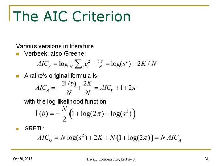
The AIC Criterion Various versions in literature n Verbeek, also Greene: n Akaike‘s original formula is with the log-likelihood function n GRETL: Oct 30, 2015 Hackl, Econometrics, Lecture 3 31

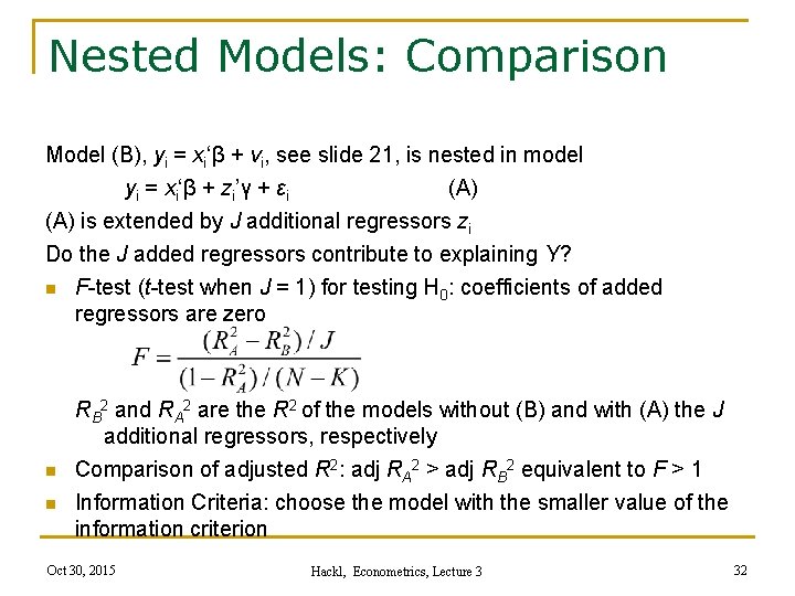
Nested Models: Comparison Model (B), yi = xi‘β + vi, see slide 21, is nested in model yi = xi‘β + zi’γ + εi (A) is extended by J additional regressors zi Do the J added regressors contribute to explaining Y? n F-test (t-test when J = 1) for testing H 0: coefficients of added regressors are zero n n RB 2 and RA 2 are the R 2 of the models without (B) and with (A) the J additional regressors, respectively Comparison of adjusted R 2: adj RA 2 > adj RB 2 equivalent to F > 1 Information Criteria: choose the model with the smaller value of the information criterion Oct 30, 2015 Hackl, Econometrics, Lecture 3 32

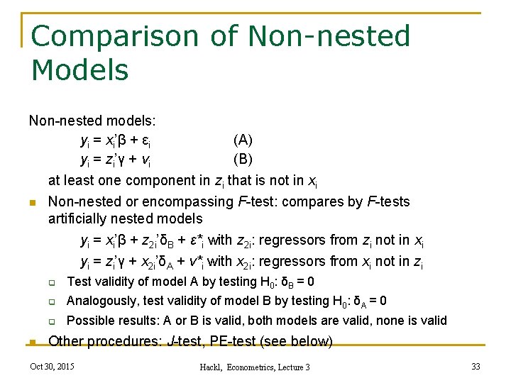
Comparison of Non-nested Models Non-nested models: yi = xi’β + εi (A) yi = zi’γ + vi (B) at least one component in zi that is not in xi n Non-nested or encompassing F-test: compares by F-tests artificially nested models yi = xi’β + z 2 i’δB + ε*i with z 2 i: regressors from zi not in xi yi = zi’γ + x 2 i’δA + v*i with x 2 i: regressors from xi not in zi n q Test validity of model A by testing H 0: δB = 0 q Analogously, test validity of model B by testing H 0: δA = 0 q Possible results: A or B is valid, both models are valid, none is valid Other procedures: J-test, PE-test (see below) Oct 30, 2015 Hackl, Econometrics, Lecture 3 33

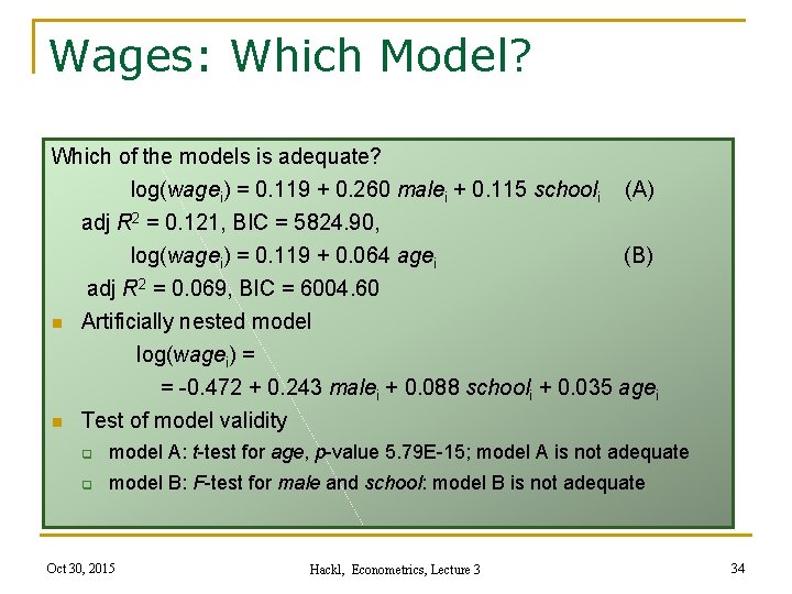
Wages: Which Model? Which of the models is adequate? log(wagei) = 0. 119 + 0. 260 malei + 0. 115 schooli n n (A) adj R 2 = 0. 121, BIC = 5824. 90, log(wagei) = 0. 119 + 0. 064 agei (B) adj R 2 = 0. 069, BIC = 6004. 60 Artificially nested model log(wagei) = = -0. 472 + 0. 243 malei + 0. 088 schooli + 0. 035 agei Test of model validity q model A: t-test for age, p-value 5. 79 E-15; model A is not adequate q model B: F-test for male and school: model B is not adequate Oct 30, 2015 Hackl, Econometrics, Lecture 3 34

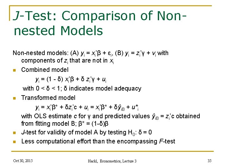
J-Test: Comparison of Nonnested Models Non-nested models: (A) yi = xi’β + εi, (B) yi = zi’γ + vi with components of zi that are not in xi n Combined model yi = (1 - δ) xi’β + δ zi’γ + ui with 0 < δ < 1; δ indicates model adequacy n Transformed model yi = xi’β* + δzi’c + ui = xi’β* + δŷi. B + u*i with OLS estimate c for γ and predicted values ŷi. B = zi’c obtained from fitting model B; β* = (1 -δ)β n J-test for validity of model A by testing H 0: δ = 0 n Less computational effort than the encompassing F-test Oct 30, 2015 Hackl, Econometrics, Lecture 3 35

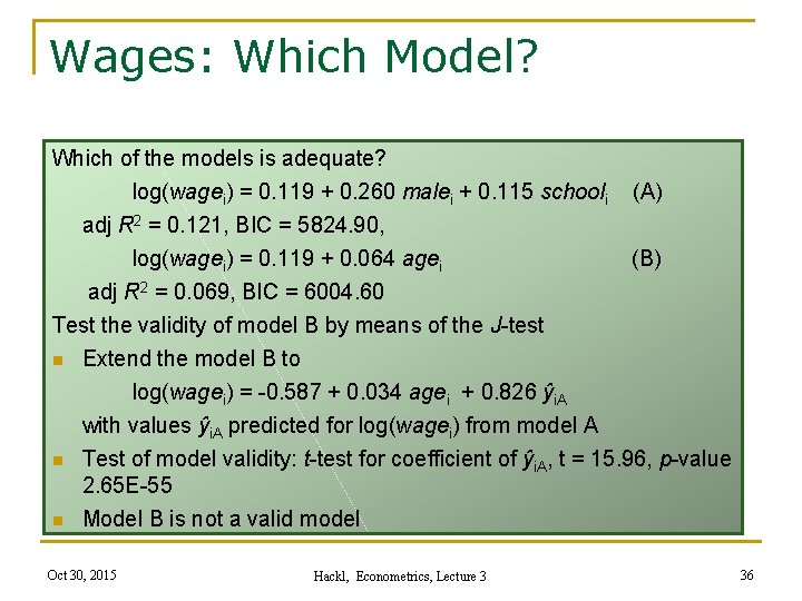
Wages: Which Model? Which of the models is adequate? log(wagei) = 0. 119 + 0. 260 malei + 0. 115 schooli adj R 2 = 0. 121, BIC = 5824. 90, log(wagei) = 0. 119 + 0. 064 agei adj R 2 = 0. 069, BIC = 6004. 60 Test the validity of model B by means of the J-test n Extend the model B to log(wagei) = -0. 587 + 0. 034 agei + 0. 826 ŷi. A n n (A) (B) with values ŷi. A predicted for log(wagei) from model A Test of model validity: t-test for coefficient of ŷi. A, t = 15. 96, p-value 2. 65 E-55 Model B is not a valid model Oct 30, 2015 Hackl, Econometrics, Lecture 3 36

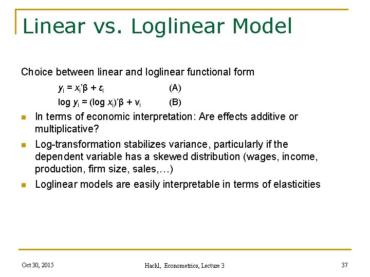
Linear vs. Loglinear Model Choice between linear and loglinear functional form n n n yi = xi’β + εi (A) log yi = (log xi)’β + vi (B) In terms of economic interpretation: Are effects additive or multiplicative? Log-transformation stabilizes variance, particularly if the dependent variable has a skewed distribution (wages, income, production, firm size, sales, …) Loglinear models are easily interpretable in terms of elasticities Oct 30, 2015 Hackl, Econometrics, Lecture 3 37

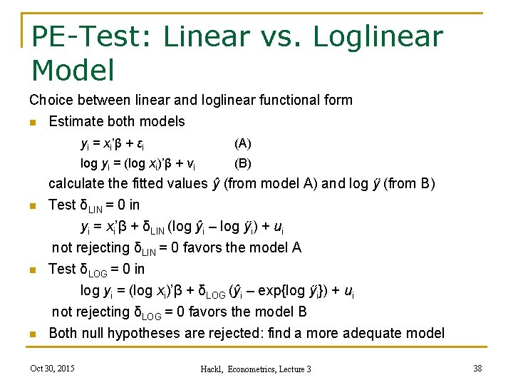
PE-Test: Linear vs. Loglinear Model Choice between linear and loglinear functional form n Estimate both models n n n yi = xi’β + εi (A) log yi = (log xi)’β + vi (B) calculate the fitted values ŷ (from model A) and log ӱ (from B) Test δLIN = 0 in yi = xi’β + δLIN (log ŷi – log ӱi) + ui not rejecting δLIN = 0 favors the model A Test δLOG = 0 in log yi = (log xi)’β + δLOG (ŷi – exp{log ӱi}) + ui not rejecting δLOG = 0 favors the model B Both null hypotheses are rejected: find a more adequate model Oct 30, 2015 Hackl, Econometrics, Lecture 3 38

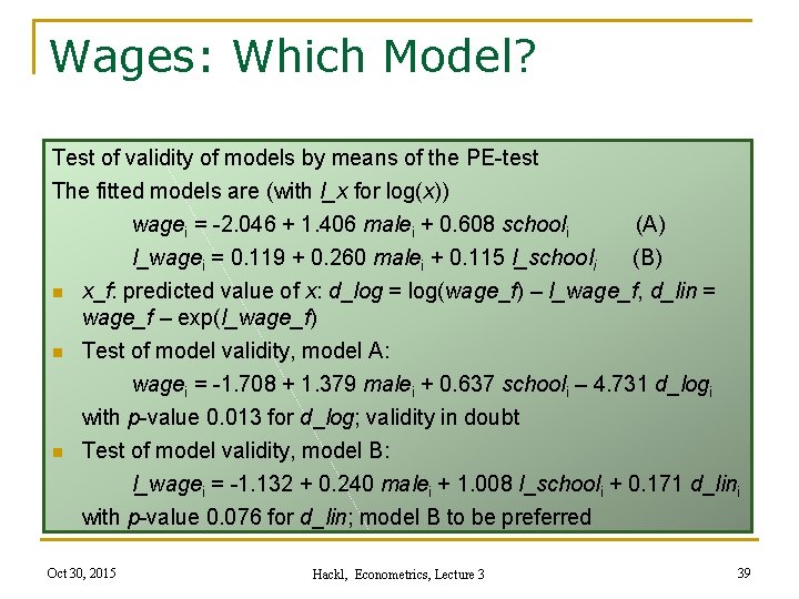
Wages: Which Model? Test of validity of models by means of the PE-test The fitted models are (with l_x for log(x)) n n n wagei = -2. 046 + 1. 406 malei + 0. 608 schooli (A) l_wagei = 0. 119 + 0. 260 malei + 0. 115 l_schooli (B) x_f: predicted value of x: d_log = log(wage_f) – l_wage_f, d_lin = wage_f – exp(l_wage_f) Test of model validity, model A: wagei = -1. 708 + 1. 379 malei + 0. 637 schooli – 4. 731 d_logi with p-value 0. 013 for d_log; validity in doubt Test of model validity, model B: l_wagei = -1. 132 + 0. 240 malei + 1. 008 l_schooli + 0. 171 d_lini with p-value 0. 076 for d_lin; model B to be preferred Oct 30, 2015 Hackl, Econometrics, Lecture 3 39

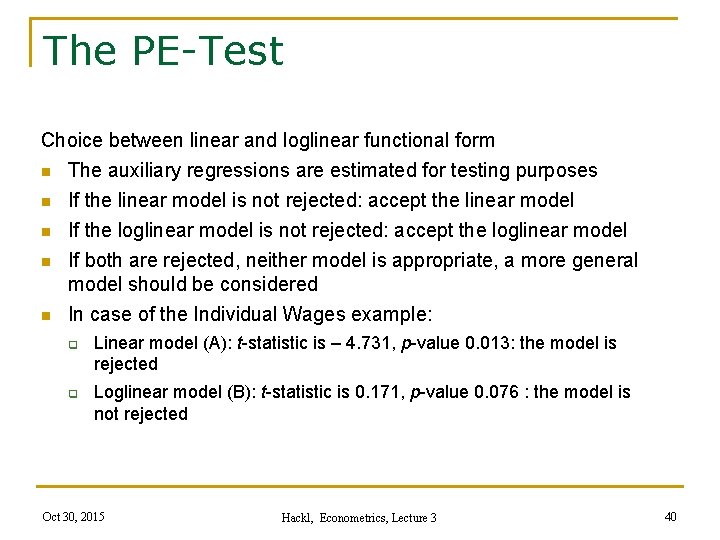
The PE-Test Choice between linear and loglinear functional form n The auxiliary regressions are estimated for testing purposes n n If the linear model is not rejected: accept the linear model If the loglinear model is not rejected: accept the loglinear model If both are rejected, neither model is appropriate, a more general model should be considered In case of the Individual Wages example: q q Linear model (A): t-statistic is – 4. 731, p-value 0. 013: the model is rejected Loglinear model (B): t-statistic is 0. 171, p-value 0. 076 : the model is not rejected Oct 30, 2015 Hackl, Econometrics, Lecture 3 40

Contents n The Linear Model: Interpretation Selection of Regressors n Specification of the Functional Form n Oct 30, 2015 Hackl, Econometrics, Lecture 3 41

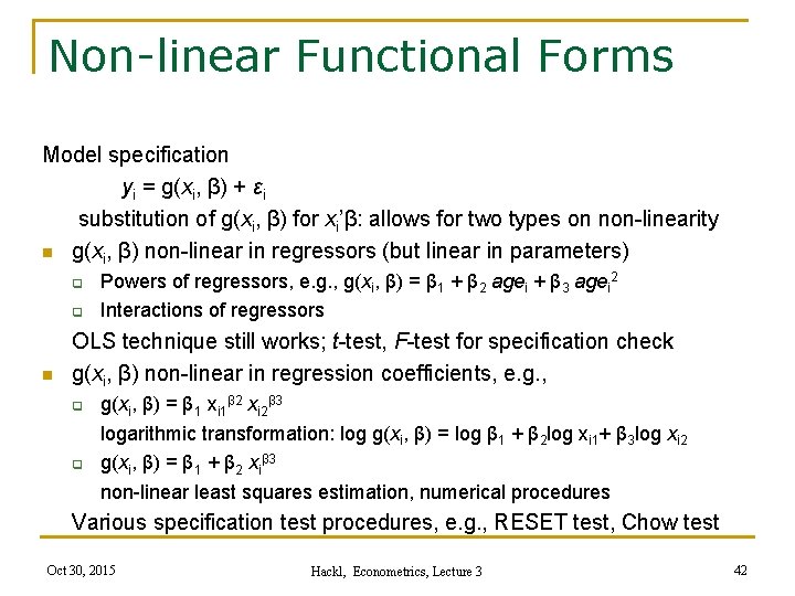
Non-linear Functional Forms Model specification yi = g(xi, β) + εi substitution of g(xi, β) for xi’β: allows for two types on non-linearity n g(xi, β) non-linear in regressors (but linear in parameters) q q n Powers of regressors, e. g. , g(xi, β) = β 1 + β 2 agei + β 3 agei 2 Interactions of regressors OLS technique still works; t-test, F-test for specification check g(xi, β) non-linear in regression coefficients, e. g. , q q g(xi, β) = β 1 xi 1β 2 xi 2β 3 logarithmic transformation: log g(xi, β) = log β 1 + β 2 log xi 1+ β 3 log xi 2 g(xi, β) = β 1 + β 2 xiβ 3 non-linear least squares estimation, numerical procedures Various specification test procedures, e. g. , RESET test, Chow test Oct 30, 2015 Hackl, Econometrics, Lecture 3 42

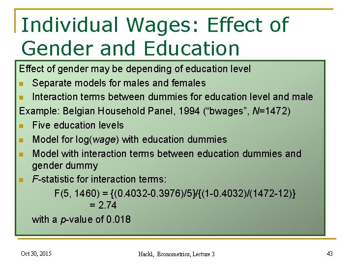
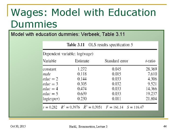
Individual Wages: Effect of Gender and Education Effect of gender may be depending of education level n Separate models for males and females n Interaction terms between dummies for education level and male Example: Belgian Household Panel, 1994 (“bwages”, N=1472) n Five education levels n Model for log(wage) with education dummies n Model with interaction terms between education dummies and gender dummy n F-statistic for interaction terms: F(5, 1460) = {(0. 4032 -0. 3976)/5}/{(1 -0. 4032)/(1472 -12)} = 2. 74 with a p-value of 0. 018 Oct 30, 2015 Hackl, Econometrics, Lecture 3 43

Wages: Model with Education Dummies Model with education dummies: Verbeek, Table 3. 11 Oct 30, 2015 Hackl, Econometrics, Lecture 3 44

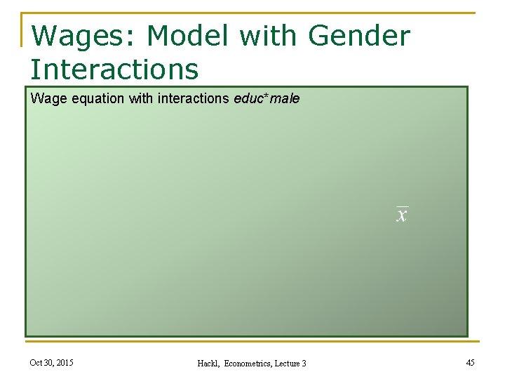
Wages: Model with Gender Interactions Wage equation with interactions educ*male Oct 30, 2015 Hackl, Econometrics, Lecture 3 45

RESET Test of the linear model E{yi |xi}= xi’β against misspecification of the functional form: n n n Null hypothesis: linear model is correct functional form Test of H 0: RESET test (Regression Equation Specification Error Test) Test idea: powers of various degrees of ŷi, the fitted values from the linear model, e. g. , ŷi², ŷi³, . . . , do not improve model fit under H 0 Test procedure: linear model extended by adding ŷi², ŷi³, . . . F- (or t-) test to decide whether powers of fitted values like ŷi², ŷi³, . . . contribute as additional regressors to explaining Y Maximal power Q of fitted values: typical choice is Q = 2 or Q = 3 Oct 30, 2015 Hackl, Econometrics, Lecture 3 46

RESET Test: The Idea Test procedure: linear model extended by adding ŷi², ŷi³, . . . n ŷi² is a function of squares (and interactions) of the regressor variables; analogously for ŷi³, . . . n If the F-test indicates that the additional regressor ŷi² contributes to explaining Y: the linear relation is not adequate, another functional form is more appropriate Oct 30, 2015 Hackl, Econometrics, Lecture 3 47

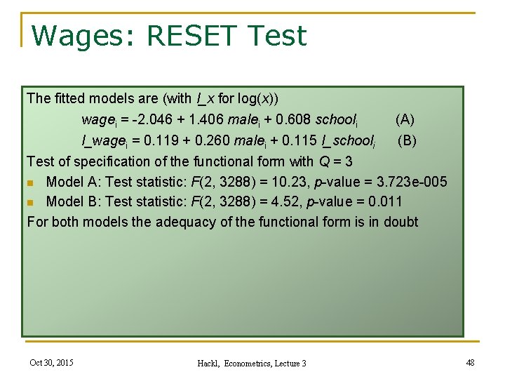
Wages: RESET Test The fitted models are (with l_x for log(x)) wagei = -2. 046 + 1. 406 malei + 0. 608 schooli (A) l_wagei = 0. 119 + 0. 260 malei + 0. 115 l_schooli (B) Test of specification of the functional form with Q = 3 n Model A: Test statistic: F(2, 3288) = 10. 23, p-value = 3. 723 e-005 n Model B: Test statistic: F(2, 3288) = 4. 52, p-value = 0. 011 For both models the adequacy of the functional form is in doubt Oct 30, 2015 Hackl, Econometrics, Lecture 3 48

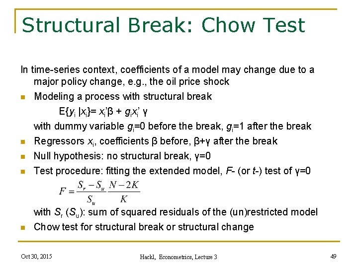
Structural Break: Chow Test In time-series context, coefficients of a model may change due to a major policy change, e. g. , the oil price shock n Modeling a process with structural break E{yi |xi}= xi’β + gixi’ γ with dummy variable gi=0 before the break, gi=1 after the break Regressors xi, coefficients β before, β+γ after the break Null hypothesis: no structural break, γ=0 Test procedure: fitting the extended model, F- (or t-) test of γ=0 n with Sr (Su): sum of squared residuals of the (un)restricted model Chow test for structural break or structural change n n n Oct 30, 2015 Hackl, Econometrics, Lecture 3 49

Chow Test: The Practice Test procedure is performed in the following steps n Fit the restricted model: Sr Fit the extended model: Su n Calculate F and the p-value from the F-distribution with K and N 2 K d. f. Needs knowledge of break point n Oct 30, 2015 Hackl, Econometrics, Lecture 3 50

Your Homework 1. Use the data set “bwages” of Verbeek for the following analyses: a) b) c) d) Estimate the model where the log hourly wages (lnwage) are explained by lnwage, male, and educ; interpret the results. Repeat exercise a) using dummy variables for the education levels, e. g. , d 1 for educ = 1, instead of the variable educ; compare the models from exercises a) and b) by using (i) the non-nested F-test and (ii) the J-test; interpret the results. Use the PE-test to decide whether the model in a) (where log hourly wages lnwage are explained) or the same model but with levels wage of hourly wages as explained variable is to be preferred; interpret the result. Repeat exercise b) with the interaction male*exper as additional regressor; interpret the result. Oct 30, 2015 Hackl, Econometrics, Lecture 3 51

Your Homework, cont’d 2. OLS is used to estimate β from yi = xi‘β + εi, but a relevant regressor zi is neglected: Show that the estimate b is biased, and derive an expression for the bias. 3. The model for a process with structural break is specified as yi = xi’β + gixi’ γ + εi, or y = Zd + ε in matrix form, with dummy variable gi=0 before the break, gi=1 after the break. Write down the design matrix Z of the model. Oct 30, 2015 Hackl, Econometrics, Lecture 3 52