Discrete Wavelet Compression of Twoway and Multiway Data

Discrete Wavelet Compression of Two-way and Multi-way Data Mohsen Kompany-Zareh, Zeinab Mokhtari, Mayam Khoshkam 09 -Nov-2011 , Tabriz Univ. 1

Signal Processing The Fourier transform Stationary Signals Non-Stationary Signals Content : Short Time Fourier Analysis (or: Gabor Transform) Wavelet Transform Discrete Wavelet Transform Continuous Wavelet Transform Example 1 Example 2. . . Example 5 2

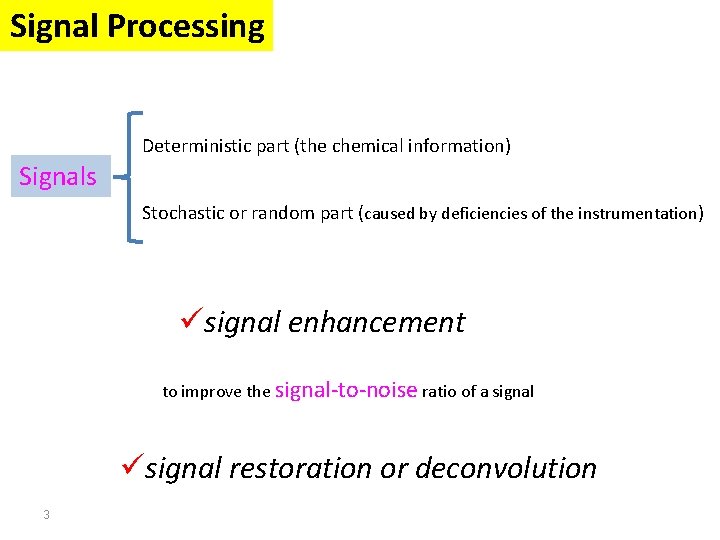
Signal Processing Deterministic part (the chemical information) Signals Stochastic or random part (caused by deficiencies of the instrumentation) üsignal enhancement to improve the signal-to-noise ratio of a signal üsignal restoration or deconvolution 3

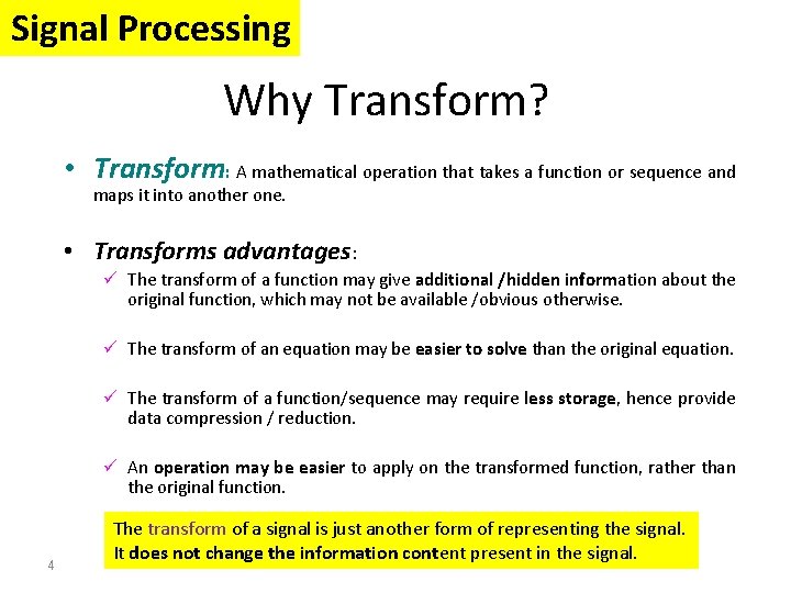
Signal Processing Why Transform? • Transform: A mathematical operation that takes a function or sequence and maps it into another one. • Transforms advantages: ü The transform of a function may give additional /hidden information about the original function, which may not be available /obvious otherwise. ü The transform of an equation may be easier to solve than the original equation. ü The transform of a function/sequence may require less storage, hence provide data compression / reduction. ü An operation may be easier to apply on the transformed function, rather than the original function. 4 The transform of a signal is just another form of representing the signal. It does not change the information content present in the signal.

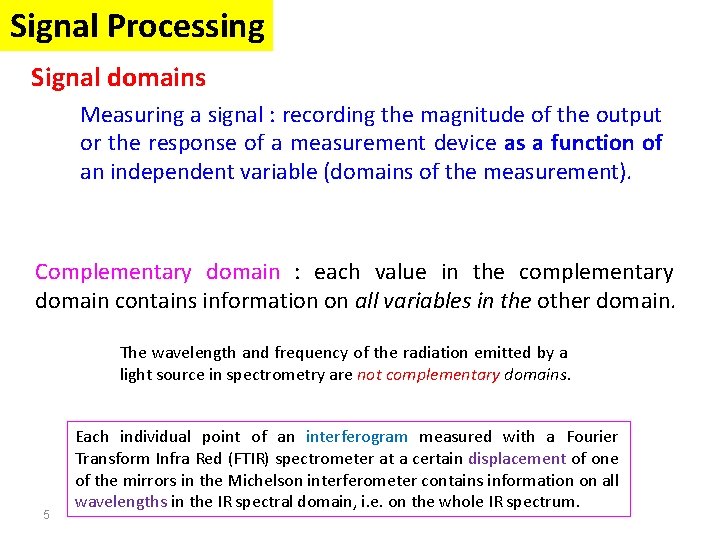
Signal Processing Signal domains Measuring a signal : recording the magnitude of the output or the response of a measurement device as a function of an independent variable (domains of the measurement). Complementary domain : each value in the complementary domain contains information on all variables in the other domain. The wavelength and frequency of the radiation emitted by a light source in spectrometry are not complementary domains. 5 Each individual point of an interferogram measured with a Fourier Transform Infra Red (FTIR) spectrometer at a certain displacement of one of the mirrors in the Michelson interferometer contains information on all wavelengths in the IR spectral domain, i. e. on the whole IR spectrum.

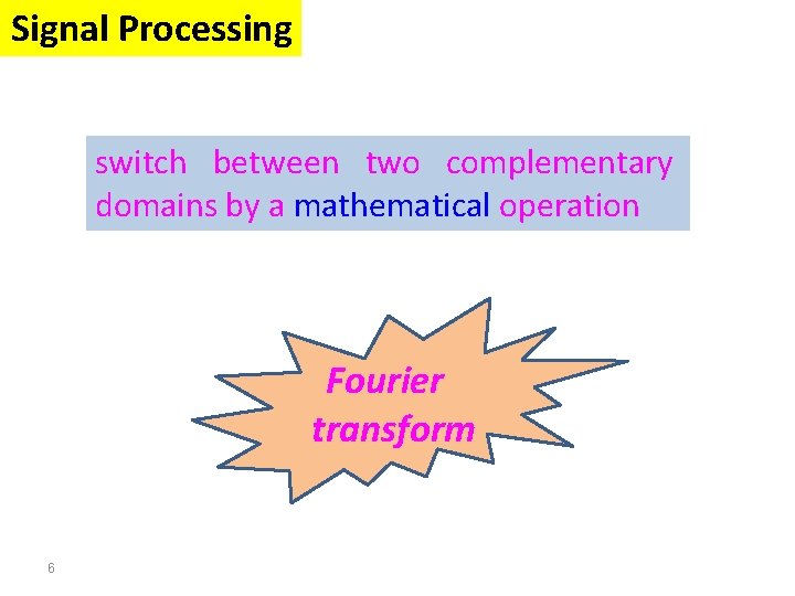
Signal Processing switch between two complementary domains by a mathematical operation Fourier transform 6

Signal Processing The Fourier transform Stationary Signals Non-Stationary Signals Content : Short Time Fourier Analysis (or: Gabor Transform) Wavelet Transform Discrete Wavelet Transform Continuous Wavelet Transform Example 1 Example 2 Example 3 7

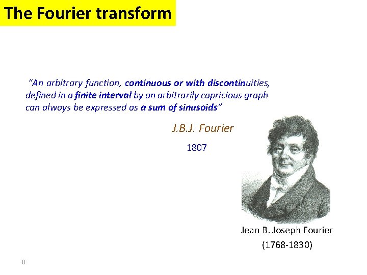
The Fourier transform “An arbitrary function, continuous or with discontinuities, defined in a finite interval by an arbitrarily capricious graph can always be expressed as a sum of sinusoids” J. B. J. Fourier 1807 Jean B. Joseph Fourier (1768 -1830) 8

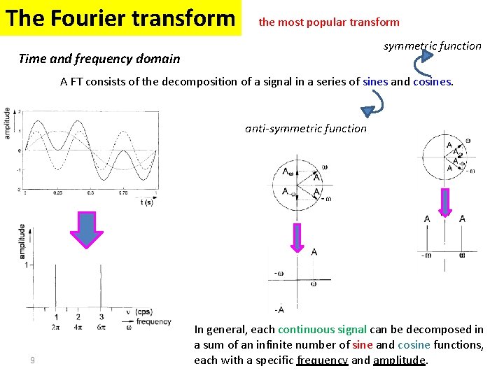
The Fourier transform the most popular transform symmetric function Time and frequency domain A FT consists of the decomposition of a signal in a series of sines and cosines. anti-symmetric function 9 In general, each continuous signal can be decomposed in a sum of an infinite number of sine and cosine functions, each with a specific frequency and amplitude.

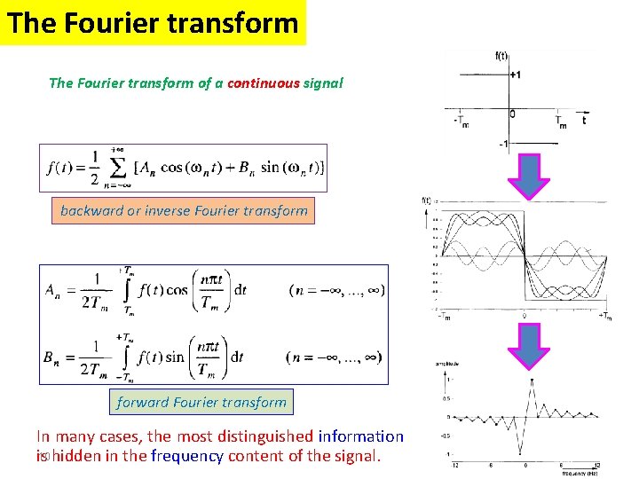
The Fourier transform of a continuous signal backward or inverse Fourier transform forward Fourier transform In many cases, the most distinguished information 10 hidden in the frequency content of the signal. is

The Fourier transform Ø FT is a reversible transform. Ø No frequency information is available in the timedomain signal. Ø No time information is available in the Fourier transformed (frequency-domain) signal. Ø Both time and frequency information are not required when the signal is so-called stationary. 11

Signal Processing The Fourier transform Stationary Signals Non-Stationary Signals Content : Short Time Fourier Analysis (or: Gabor Transform) Wavelet Transform Discrete Wavelet Transform Continuous Wavelet Transform Example 1 Example 2 Example 3 12

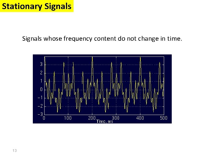
Stationary Signals whose frequency content do not change in time. 13

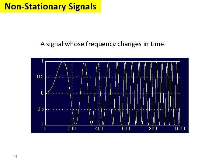
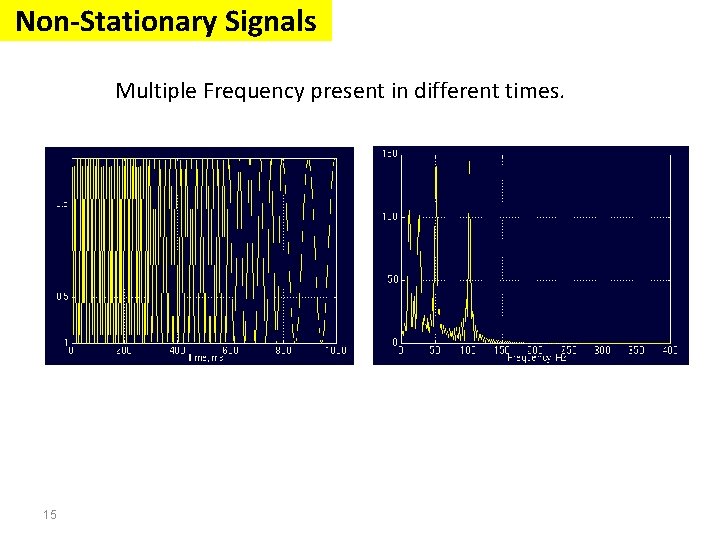
Non-Stationary Signals A signal whose frequency changes in time. 14

Non-Stationary Signals Multiple Frequency present in different times. 15

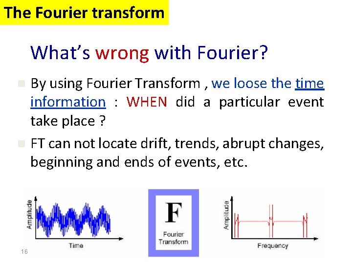
The Fourier transform What’s wrong with Fourier? By using Fourier Transform , we loose the time information : WHEN did a particular event take place ? n FT can not locate drift, trends, abrupt changes, beginning and ends of events, etc. n 16

The Fourier transform • FT is not a suitable technique for non-stationary signals. • FT gives what frequency components (spectral components) exist in the signal. Nothing more, nothing less. • When the time localization of the spectral components are needed, a transform giving the TIME-FREQUENCY REPRESENTATION of the signal is needed. 17

Signal Processing The Fourier transform Stationary Signals Non-Stationary Signals Content : Short Time Fourier Analysis (or: Gabor Transform) Wavelet Transform Discrete Wavelet Transform Continuous Wavelet Transform Example 1 Example 2 Example 3 18

Short Time Fourier Analysis (or: Gabor Transform) • How are we going to insert this time business into our frequency plots? • Can we assume that, some portion of a non -stationary signal is stationary? • If this region where the signal can be assumed to be stationary is too small, then we look at that signal from narrow windows, narrow enough that the portion of the signal seen from these windows are indeed stationary. 19

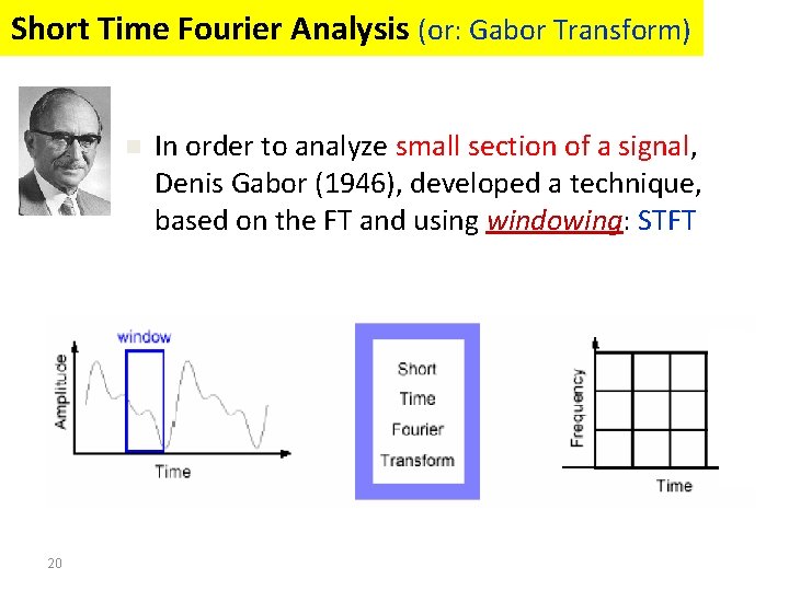
Short Time Fourier Analysis (or: Gabor Transform) n 20 In order to analyze small section of a signal, Denis Gabor (1946), developed a technique, based on the FT and using windowing: STFT

Short Time Fourier Analysis (or: Gabor Transform) o A compromise between time-based and frequency-based views of a signal. o Both time and frequency are represented in limited precision. o The precision is determined by the size of the window. o Once you choose a particular size for the time window - it will be the same for all frequencies. 21

Short Time Fourier Analysis (or: Gabor Transform) What’s wrong with Gabor? n 22 Many signals require a more flexible approach - so we can vary the window size to determine more accurately either time or frequency.

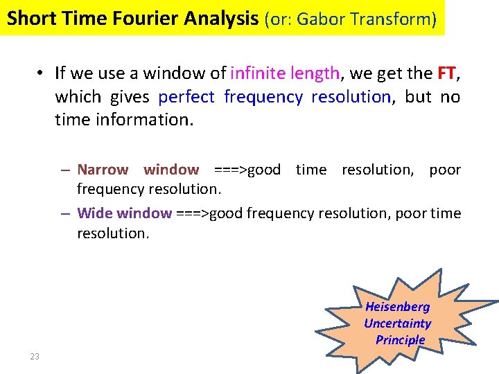
Short Time Fourier Analysis (or: Gabor Transform) • If we use a window of infinite length, we get the FT, which gives perfect frequency resolution, but no time information. – Narrow window ===>good time resolution, poor frequency resolution. – Wide window ===>good frequency resolution, poor time resolution. Heisenberg Uncertainty Principle 23

Signal Processing The Fourier transform Stationary Signals Non-Stationary Signals Content : Short Time Fourier Analysis (or: Gabor Transform) Wavelet Transform Discrete Wavelet Transform Continuous Wavelet Transform Example 1 Example 2 Example 3 24

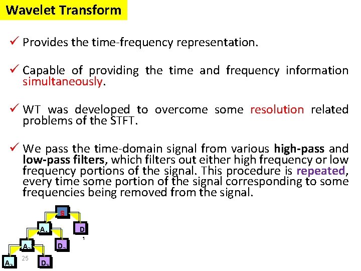
Wavelet Transform ü Provides the time-frequency representation. ü Capable of providing the time and frequency information simultaneously. ü WT was developed to overcome some resolution related problems of the STFT. ü We pass the time-domain signal from various high-pass and low-pass filters, which filters out either high frequency or low frequency portions of the signal. This procedure is repeated, every time some portion of the signal corresponding to some frequencies being removed from the signal. S D A 1 1 D 2 A 3 25 D 3

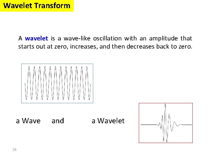
Wavelet Transform A wavelet is a wave-like oscillation with an amplitude that starts out at zero, increases, and then decreases back to zero. a Wave 26 and a Wavelet

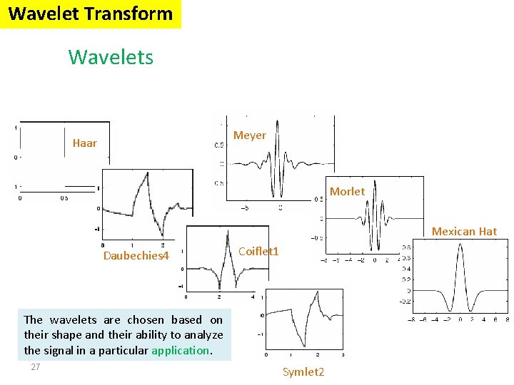
Wavelet Transform Wavelets Meyer Haar Morlet Mexican Hat Daubechies 4 Coiflet 1 The wavelets are chosen based on their shape and their ability to analyze the signal in a particular application. 27 Symlet 2

Wavelet Transform ØThe Wavelet Transform provides a time-frequency representation of the signal. ØIt was developed to overcome the short coming of the Short Time Fourier Transform (STFT), which can also be used to analyze nonstationary signals. ØThe wavelet analysis is done similar to the STFT analysis. ØThe signal to be analyzed is multiplied with a wavelet function just as it is multiplied with a window function in STFT, and then the transform is computed for each segment generated. ØHowever, unlike STFT, in Wavelet Transform, the width of the wavelet function changes with each spectral component. 28

Signal Processing The Fourier transform Stationary Signals Non-Stationary Signals Content : Short Time Fourier Analysis (or: Gabor Transform) Wavelet Transform Discrete Wavelet Transform Continuous Wavelet Transform Example 1 Example 2 Example 3 29

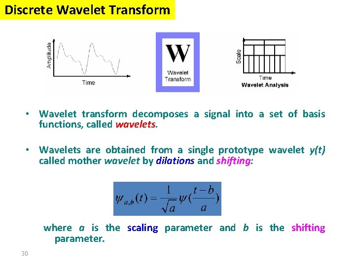
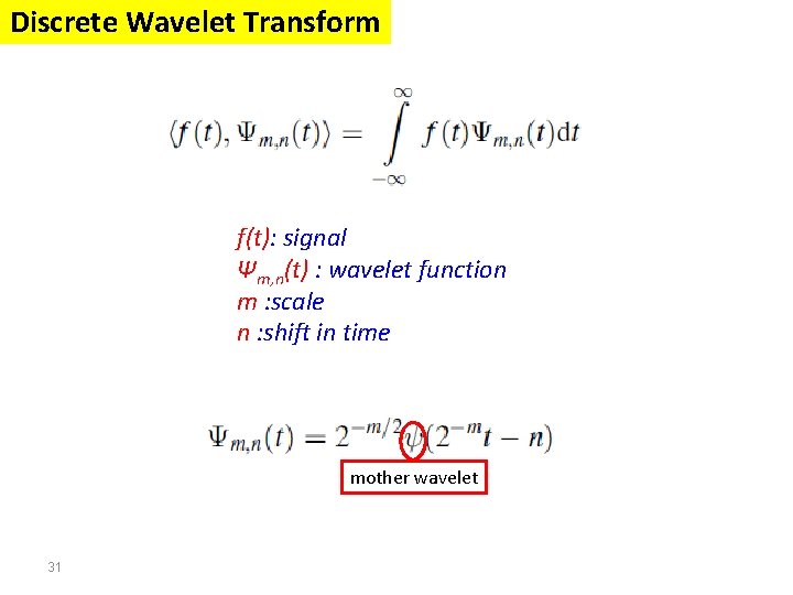
Discrete Wavelet Transform • Wavelet transform decomposes a signal into a set of basis functions, called wavelets. • Wavelets are obtained from a single prototype wavelet y(t) called mother wavelet by dilations and shifting: where a is the scaling parameter and b is the shifting parameter. 30

Discrete Wavelet Transform f(t): signal Ψm, n(t) : wavelet function m : scale n : shift in time mother wavelet 31

Discrete Wavelet Transform To transform measurements available in a discrete form a discrete wavelet transform (DWT) is applied. Condition is that the number of data is equal to 2 n. In the discrete wavelet transform the analyzing wavelet is represented by a number of coefficients, called wavelet filter coefficients. Generally, the wavelet member n is characterized by 2 n coefficients. The value of n defines the level of the wavelet. For instance, for n = 2 the level 2 wavelet is obtained. For each level, a transform matrix is defined in which the wavelet filter coefficients are arranged in a specific way. The level zero (1 non-zero coefficient) returns the signal itself. The widest wavelet considered is the one for which 2 n is equal to N, the number of measurements. 32

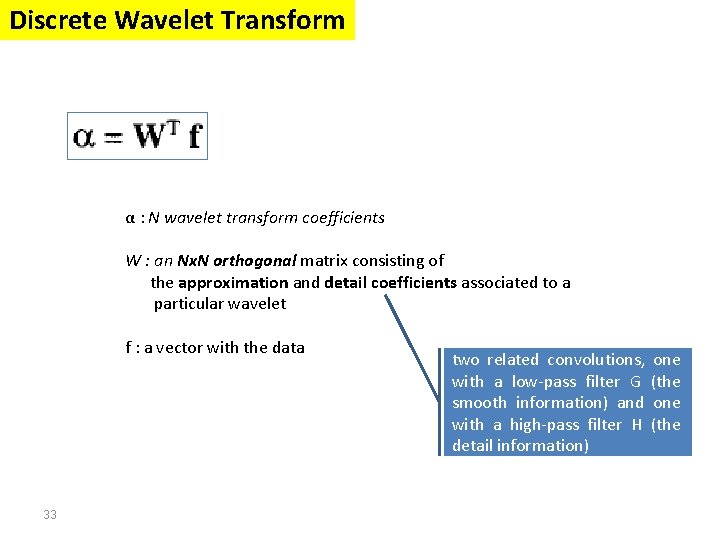
Discrete Wavelet Transform α : N wavelet transform coefficients W : an Nx. N orthogonal matrix consisting of the approximation and detail coefficients associated to a particular wavelet f : a vector with the data 33 two related convolutions, with a low-pass filter G smooth information) and with a high-pass filter H detail information) one (the

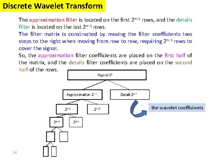
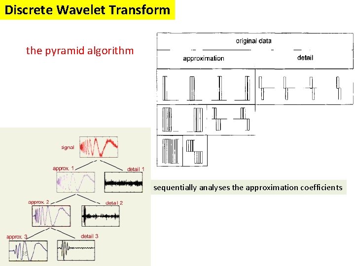
Discrete Wavelet Transform The approximation filter is located on the first 2 n− 1 rows, and the details filter is located on the last 2 n− 1 rows. The filter matrix is constructed by moving the filter coefficients two steps to the right when moving from row to row, requiring 2 n− 1 rows to cover the signal. So, the approximation filter coefficients are placed on the first half of the matrix, and the details filter coefficients are placed on the second half of the rows. the wavelet coefficients 34

Discrete Wavelet Transform the pyramid algorithm sequentially analyses the approximation coefficients 35

Signal Processing The Fourier transform Stationary Signals Non-Stationary Signals Content : Short Time Fourier Analysis (or: Gabor Transform) Wavelet Transform Discrete Wavelet Transform Continuous Wavelet Transform Example 1 Example 2 Example 3 36

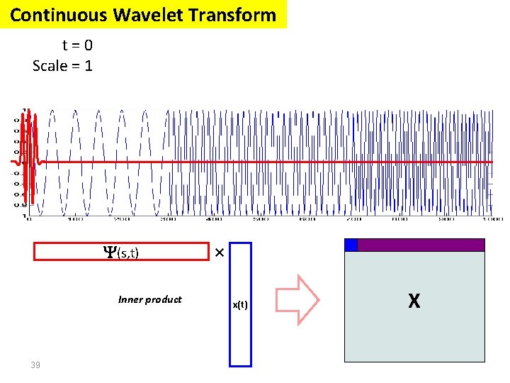
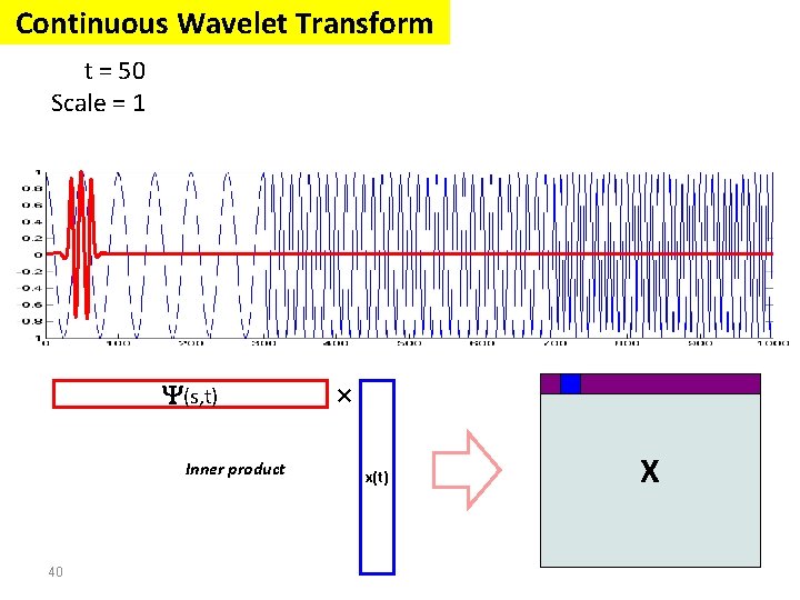
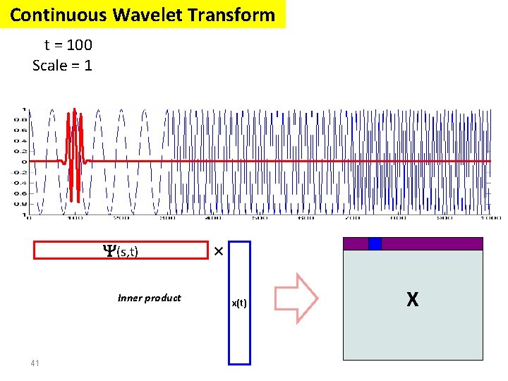
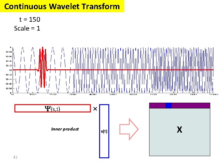
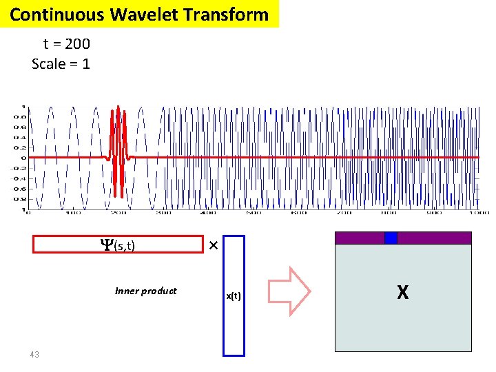
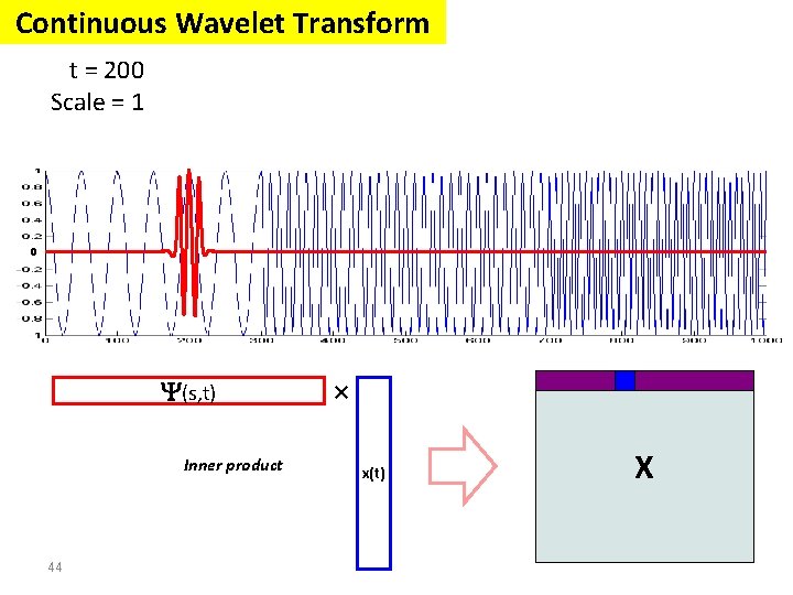
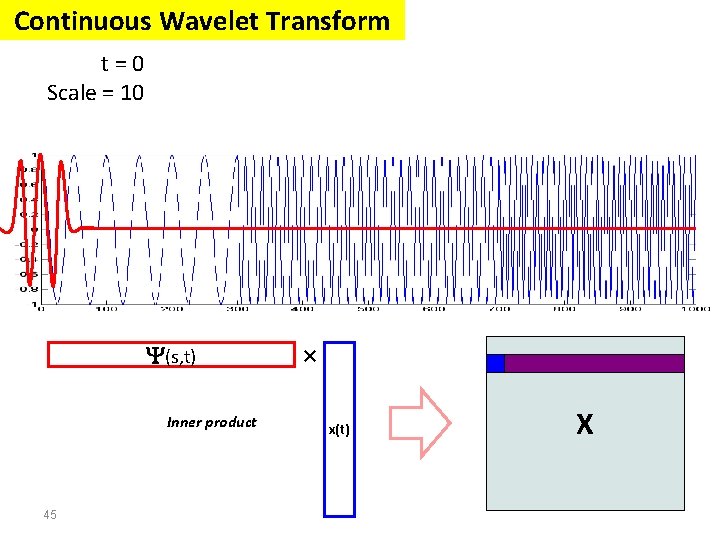
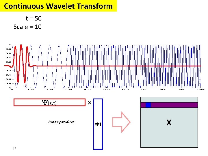
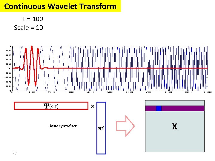
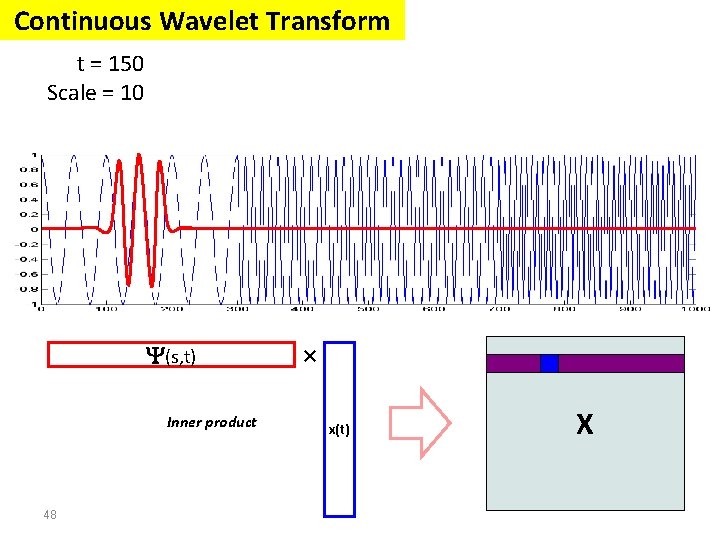
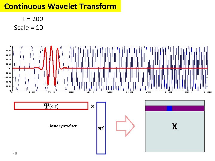
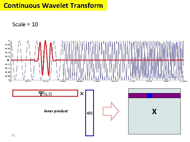
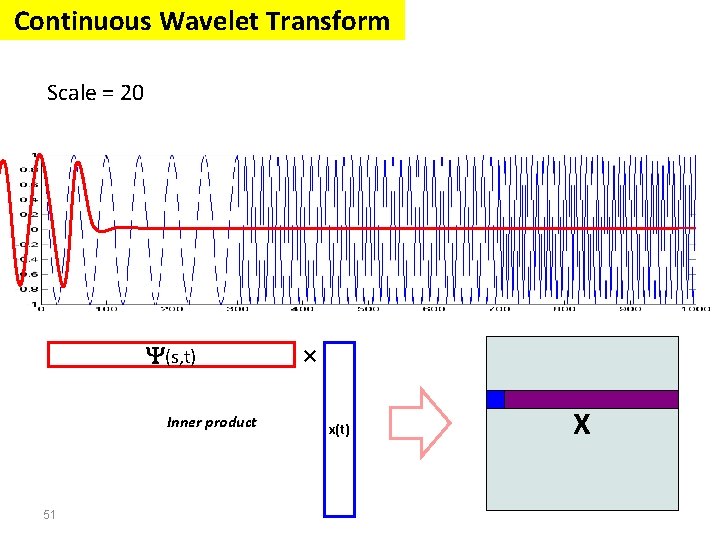
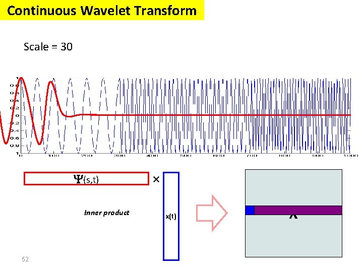
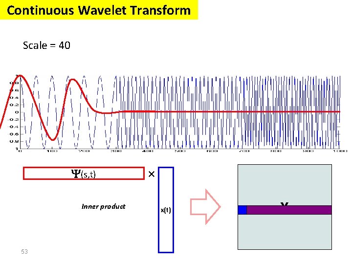
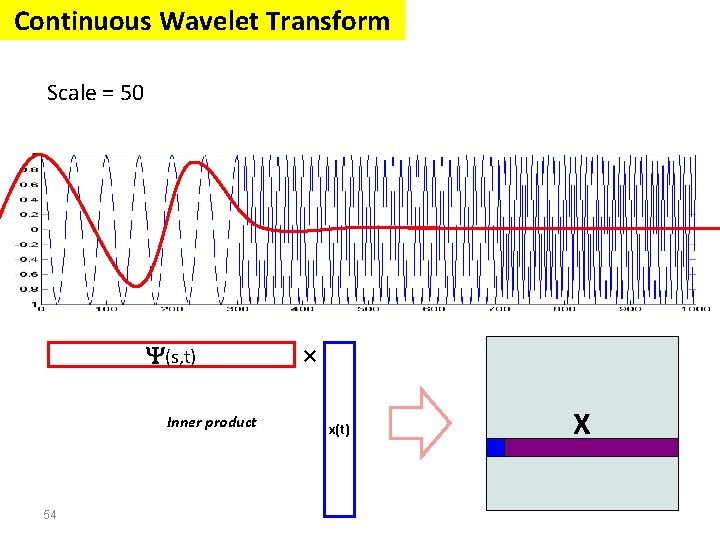
Continuous Wavelet Transform The continuous wavelet transform was developed as an alternative approach to the STFT (short time Fourier transform) to overcome the resolution problem. The wavelet analysis is done in a similar way to the STFT analysis, in the sense that the signal is multiplied with a function, wavelet, similar to the window function in the STFT, and the transform is computed separately for different segments of the time domain signal. 37

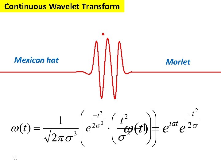
Continuous Wavelet Transform Mexican hat 38 Morlet

Continuous Wavelet Transform t=0 Scale = 1 (s, t) Inner product 39 × x(t) X

Continuous Wavelet Transform t = 50 Scale = 1 (s, t) Inner product 40 × x(t) X

Continuous Wavelet Transform t = 100 Scale = 1 (s, t) Inner product 41 × x(t) X

Continuous Wavelet Transform t = 150 Scale = 1 (s, t) Inner product 42 × x(t) X

Continuous Wavelet Transform t = 200 Scale = 1 (s, t) Inner product 43 × x(t) X

Continuous Wavelet Transform t = 200 Scale = 1 0 (s, t) Inner product 44 × x(t) X

Continuous Wavelet Transform t=0 Scale = 10 (s, t) Inner product 45 × x(t) X

Continuous Wavelet Transform t = 50 Scale = 10 (s, t) Inner product 46 × x(t) X

Continuous Wavelet Transform t = 100 Scale = 10 (s, t) Inner product 47 × x(t) X

Continuous Wavelet Transform t = 150 Scale = 10 (s, t) Inner product 48 × x(t) X

Continuous Wavelet Transform t = 200 Scale = 10 (s, t) Inner product 49 × x(t) X

Continuous Wavelet Transform Scale = 10 0 (s, t) Inner product 50 × x(t) X

Continuous Wavelet Transform Scale = 20 (s, t) Inner product 51 × x(t) X

Continuous Wavelet Transform Scale = 30 (s, t) Inner product 52 × x(t) X

Continuous Wavelet Transform Scale = 40 (s, t) Inner product 53 × x(t) X

Continuous Wavelet Transform Scale = 50 (s, t) Inner product 54 × x(t) X

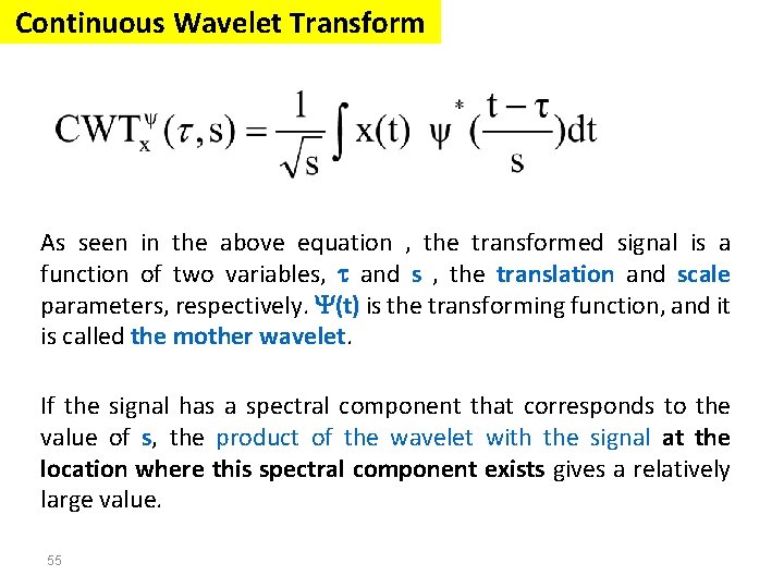
Continuous Wavelet Transform As seen in the above equation , the transformed signal is a function of two variables, and s , the translation and scale parameters, respectively. (t) is the transforming function, and it is called the mother wavelet. If the signal has a spectral component that corresponds to the value of s, the product of the wavelet with the signal at the location where this spectral component exists gives a relatively large value. 55

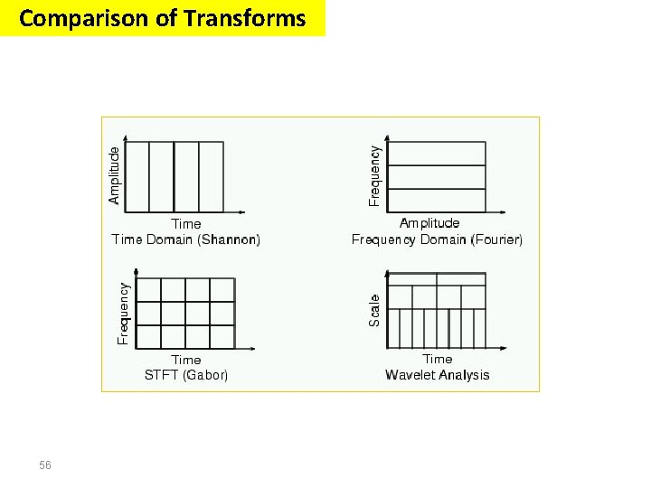
Comparison of Transforms 56

Signal Processing The Fourier transform Stationary Signals Non-Stationary Signals Content : Short Time Fourier Analysis (or: Gabor Transform) Wavelet Transform Discrete Wavelet Transform Continuous Wavelet Transform Example 1 Example 2 Example 3 57

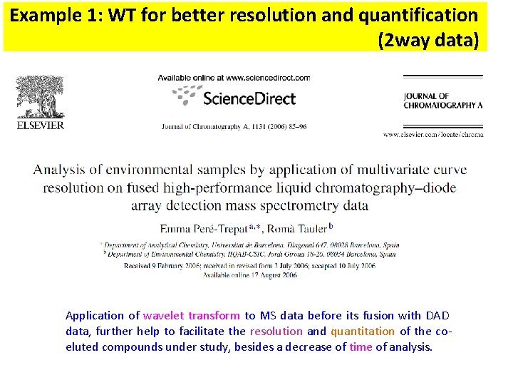
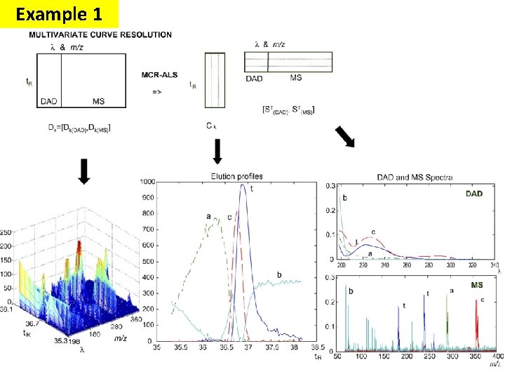
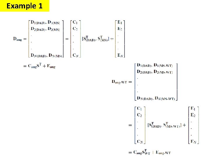
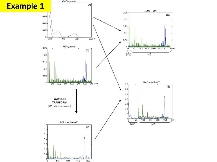
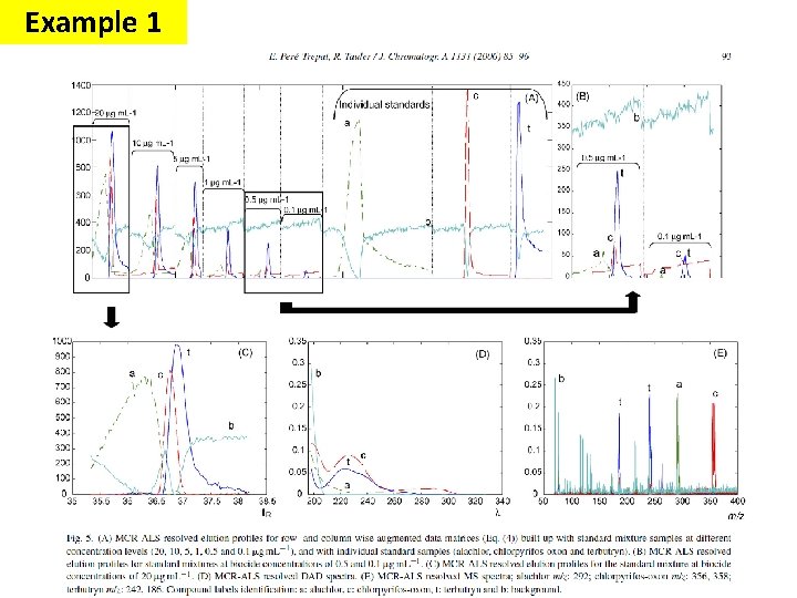
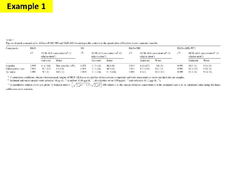
Example 1: WT for better resolution and quantification (2 way data) Application of wavelet transform to MS data before its fusion with DAD data, further help to facilitate the resolution and quantitation of the coeluted compounds under study, besides a decrease of time of analysis.

Example 1

Example 1

Example 1

Example 1

Example 1

Example 1

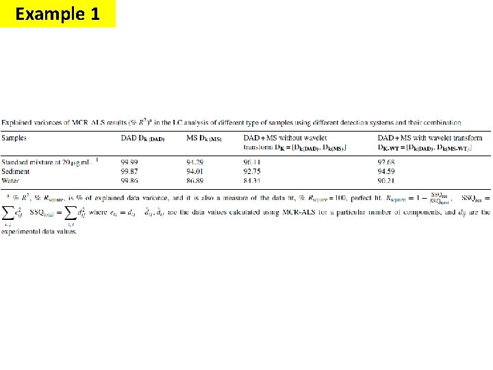
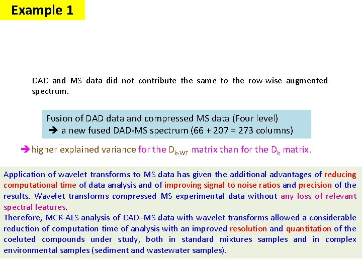
Example 1 DAD and MS data did not contribute the same to the row-wise augmented spectrum. Fusion of DAD data and compressed MS data (Four level) a new fused DAD-MS spectrum (66 + 207 = 273 columns) higher explained variance for the Dk-WT matrix than for the Dk matrix. Application of wavelet transforms to MS data has given the additional advantages of reducing computational time of data analysis and of improving signal to noise ratios and precision of the results. Wavelet transforms compressed MS experimental data without any loss of relevant spectral features. Therefore, MCR-ALS analysis of DAD–MS data with wavelet transforms allowed a considerable reduction of computation time of analysis with an improved resolution and quantitation of the coeluted compounds under study, both in standard mixtures samples and in complex environmental samples (sediment and wastewater samples).

Signal Processing The Fourier transform Stationary Signals Non-Stationary Signals Content : Short Time Fourier Analysis (or: Gabor Transform) Wavelet Transform Discrete Wavelet Transform Continuous Wavelet Transform Example 1 Example 2 Example 3 66

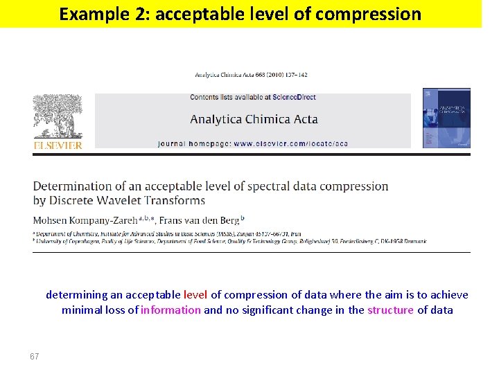
Example 2: acceptable level of compression determining an acceptable level of compression of data where the aim is to achieve minimal loss of information and no significant change in the structure of data 67

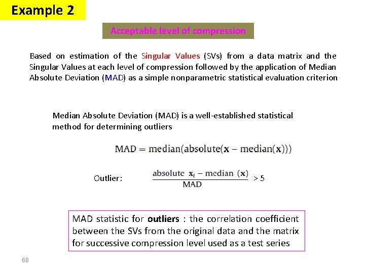
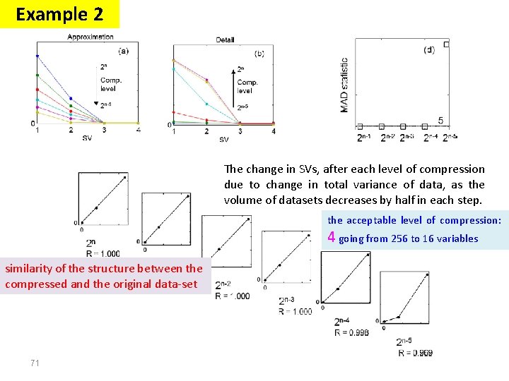
Example 2 Acceptable level of compression Based on estimation of the Singular Values (SVs) from a data matrix and the Singular Values at each level of compression followed by the application of Median Absolute Deviation (MAD) as a simple nonparametric statistical evaluation criterion Median Absolute Deviation (MAD) is a well-established statistical method for determining outliers Outlier: >5 MAD statistic for outliers : the correlation coefficient between the SVs from the original data and the matrix for successive compression level used as a test series 68

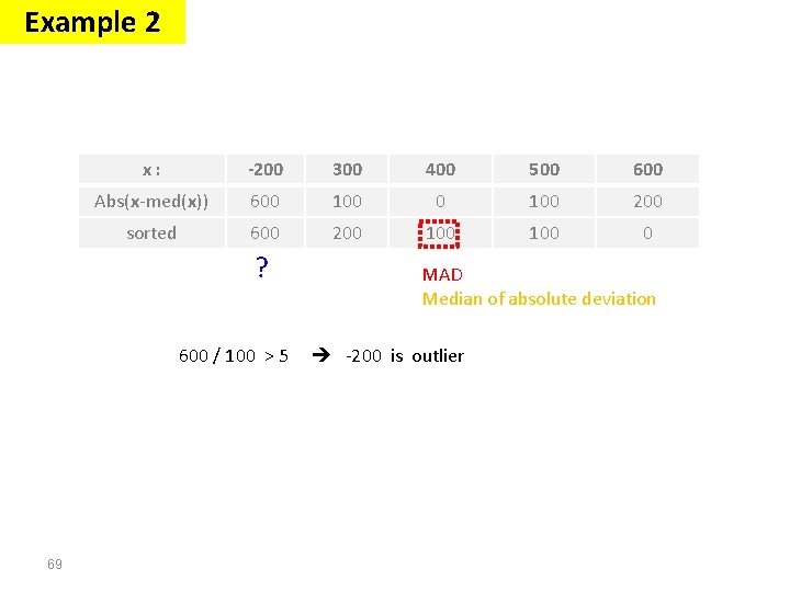
Example 2 x: -200 300 400 500 600 Abs(x-med(x)) 600 100 200 sorted 600 200 100 0 ? 600 / 100 > 5 69 MAD Median of absolute deviation -200 is outlier

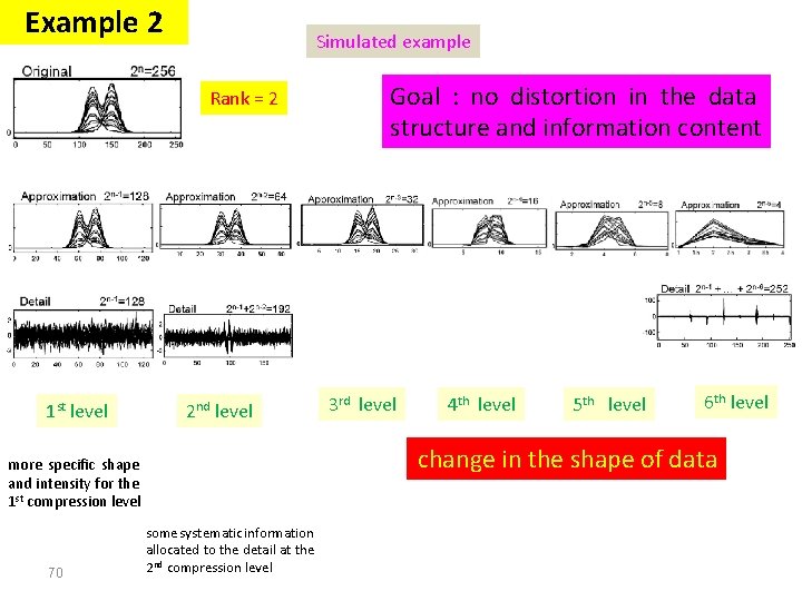
Example 2 Simulated example Rank = 2 1 st level 2 nd level 3 rd level 4 th level 5 th level 6 th level change in the shape of data more specific shape and intensity for the 1 st compression level 70 Goal : no distortion in the data structure and information content some systematic information allocated to the detail at the 2 nd compression level

Example 2 The change in SVs, after each level of compression due to change in total variance of data, as the volume of datasets decreases by half in each step. the acceptable level of compression: 4 going from 256 to 16 variables similarity of the structure between the compressed and the original data-set 71

Example 2 Some points: The effective rank of the data needs to be two or more. To make the MAD test applicable at least three levels of compression are required. From the third level of compression onwards we add each successive level in steps and we stop compression when we find that a clear change in SV plot has appeared. 72

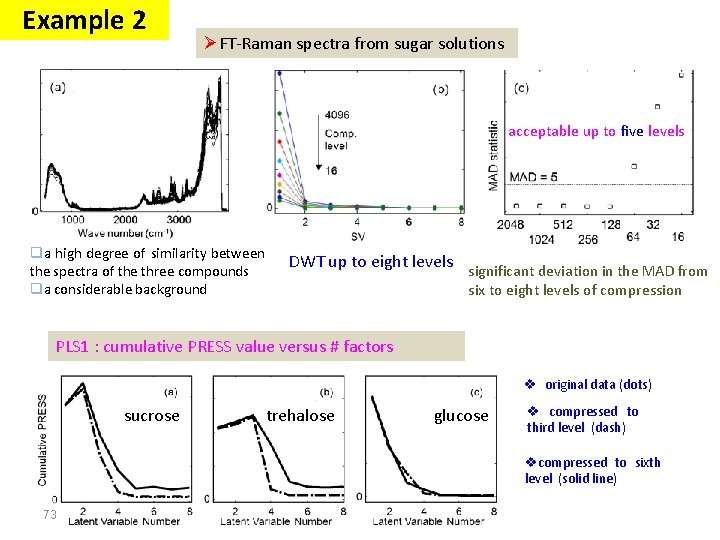
Example 2 ØFT-Raman spectra from sugar solutions acceptable up to five levels qa high degree of similarity between the spectra of the three compounds qa considerable background DWT up to eight levels significant deviation in the MAD from six to eight levels of compression PLS 1 : cumulative PRESS value versus # factors v original data (dots) sucrose trehalose glucose v compressed to third level (dash) vcompressed to sixth level (solid line) 73

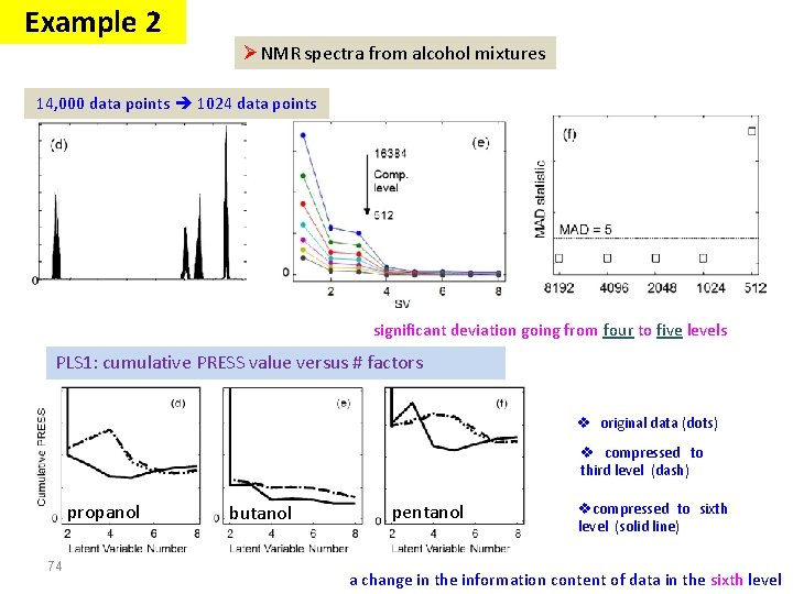
Example 2 ØNMR spectra from alcohol mixtures 14, 000 data points 1024 data points significant deviation going from four to five levels PLS 1: cumulative PRESS value versus # factors v original data (dots) v compressed to third level (dash) propanol 74 butanol pentanol vcompressed to sixth level (solid line) a change in the information content of data in the sixth level

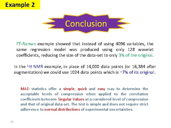
Example 2 Conclusion FT-Raman example showed that instead of using 4096 variables, the same regression model was produced using only 128 wavelet coefficients, reducing the size of the data-set to only 3% of the original. In the 1 H NMR example, in place of 14, 000 data points (or 16, 384 after augmentation) we could use 1024 data points which is ∼ 7% of its original. MAD statistics offer a simple, quick and easy way to determine the acceptable levels of compression when applied to the correlation coefficients between Singular Values at a considered level of compression and that of original data-set. The test is simple and does not require strict adherence to normal distributions of experimental uncertainties. 75

Signal Processing The Fourier transform Stationary Signals Non-Stationary Signals Content : Short Time Fourier Analysis (or: Gabor Transform) Wavelet Transform Discrete Wavelet Transform Continuous Wavelet Transform Example 1 Example 2 Example 3 76

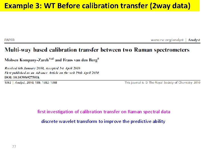
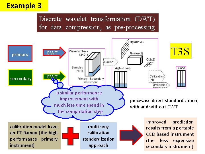
Example 3: WT Before calibration transfer (2 way data) first investigation of calibration transfer on Raman spectral data discrete wavelet transform to improve the predictive ability 77

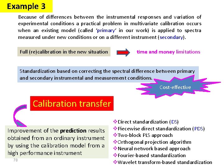
Example 3 Because of differences between the instrumental responses and variation of experimental conditions a practical problem in multivariate calibration occurs when an existing model (called ‘primary’ in our work) is applied to spectra measured under new conditions or on a different instrument (secondary). Full (re)calibration in the new situation time and money limitations Standardization based on correcting the spectral difference between primary and secondary instrumental and measurement conditions. Cost-effective Calibration transfer Improvement of the prediction results obtained from an ordinary instrument by using the calibration model from a high performance instrument 78 v. Direct standardization (DS) v. Piecewise direct standardization (PDS) v. Two-block PLS approach v. Orthogonal projection algorithm v. Neural network based approach v. Fourier-based standardization v. Wavelet transform-based standardization

Example 3 Discrete wavelet transformation (DWT) for data compression, as pre-processing method primary DWT secondary DWT T 3 S a similar performance improvement with much less time spend in the computation step calibration model from an FT-Raman (the high performance primary instrument) 79 multi-way calibration standardization approach piecewise direct standardization, with and without DWT Improved prediction results from a portable CCD based instrument (the less expensive secondary instrument)

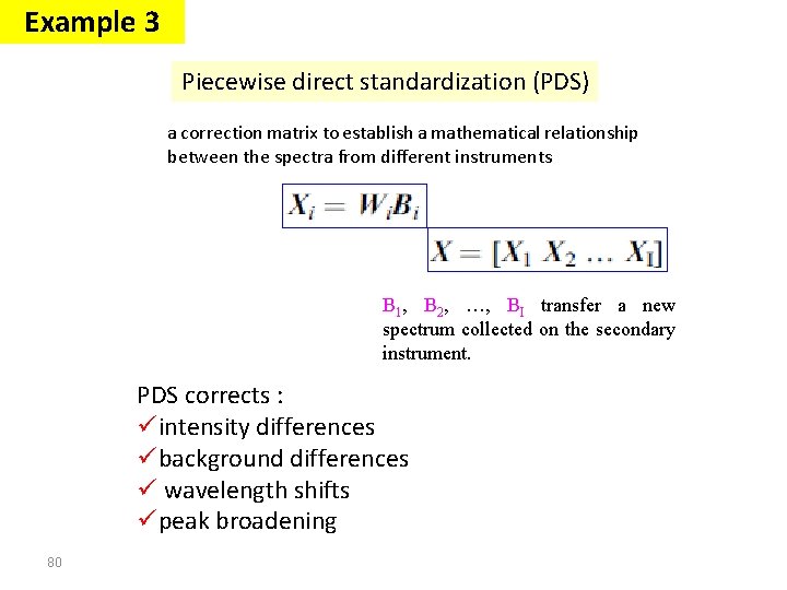
Example 3 Piecewise direct standardization (PDS) a correction matrix to establish a mathematical relationship between the spectra from different instruments B 1, B 2, …, BI transfer a new spectrum collected on the secondary instrument. PDS corrects : üintensity differences übackground differences ü wavelength shifts üpeak broadening 80

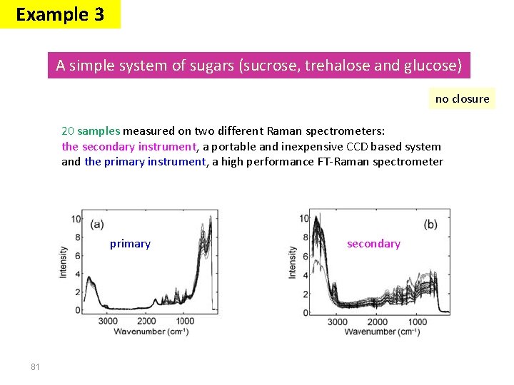
Example 3 A simple system of sugars (sucrose, trehalose and glucose) no closure 20 samples measured on two different Raman spectrometers: the secondary instrument, a portable and inexpensive CCD based system and the primary instrument, a high performance FT-Raman spectrometer primary 81 secondary

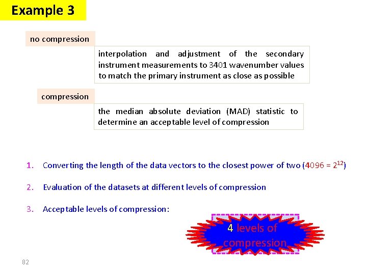
Example 3 no compression interpolation and adjustment of the secondary instrument measurements to 3401 wavenumber values to match the primary instrument as close as possible compression the median absolute deviation (MAD) statistic to determine an acceptable level of compression 1. Converting the length of the data vectors to the closest power of two (4096 = 212) 2. Evaluation of the datasets at different levels of compression 3. Acceptable levels of compression: Primary 4 levels: of 5 compression Secondary : 7 82

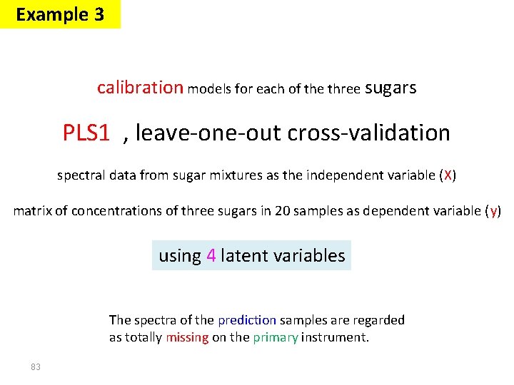
Example 3 calibration models for each of the three sugars PLS 1 , leave-one-out cross-validation spectral data from sugar mixtures as the independent variable (X) matrix of concentrations of three sugars in 20 samples as dependent variable (y) using 4 latent variables The spectra of the prediction samples are regarded as totally missing on the primary instrument. 83

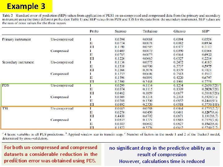
Example 3 For both un-compressed and compressed datasets a considerable reduction in the 84 prediction error was obtained using PDS. no significant drop in the predictive ability as a result of compression However, calculations time is reduced

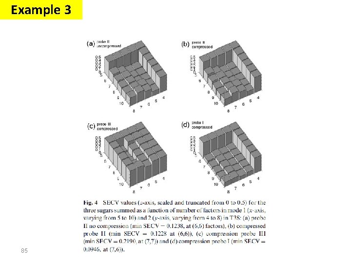
Example 3 85

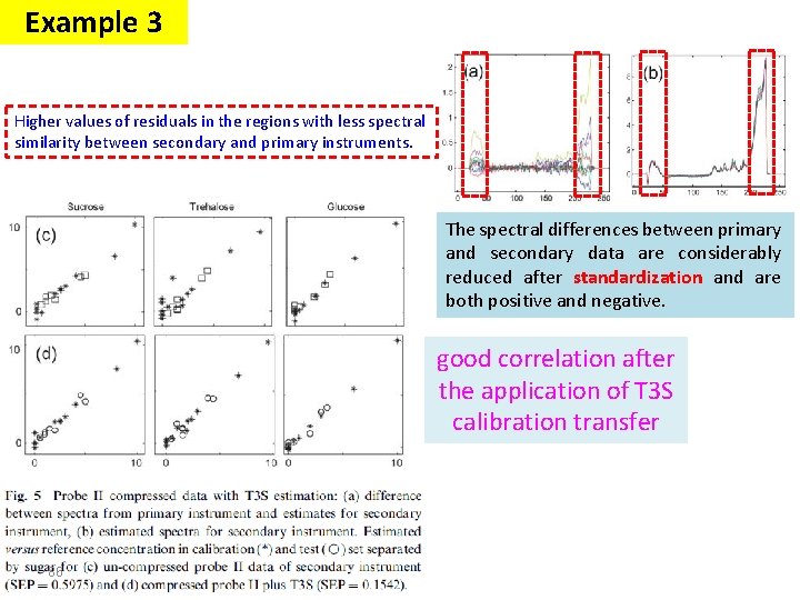
Example 3 Higher values of residuals in the regions with less spectral similarity between secondary and primary instruments. The spectral differences between primary and secondary data are considerably reduced after standardization and are both positive and negative. good correlation after the application of T 3 S calibration transfer 86

Example 3 Conclusion A compression of the data by discrete wavelet transform did not result into a better prediction, but reduced the time consumption for calculations by imputation considerably without loss of performance (going from 30 seconds to less then 5 seconds on a process computer, enabling ‘‘realtime’’ process monitoring). When the number of times of measurements and computations are very large this reduction in processing time becomes remarkable. 87

Signal Processing The Fourier transform Stationary Signals Non-Stationary Signals Content : Short Time Fourier Analysis (or: Gabor Transform) Wavelet Transform Discrete Wavelet Transform Continuous Wavelet Transform Example 1 Example 2 Example 4 88

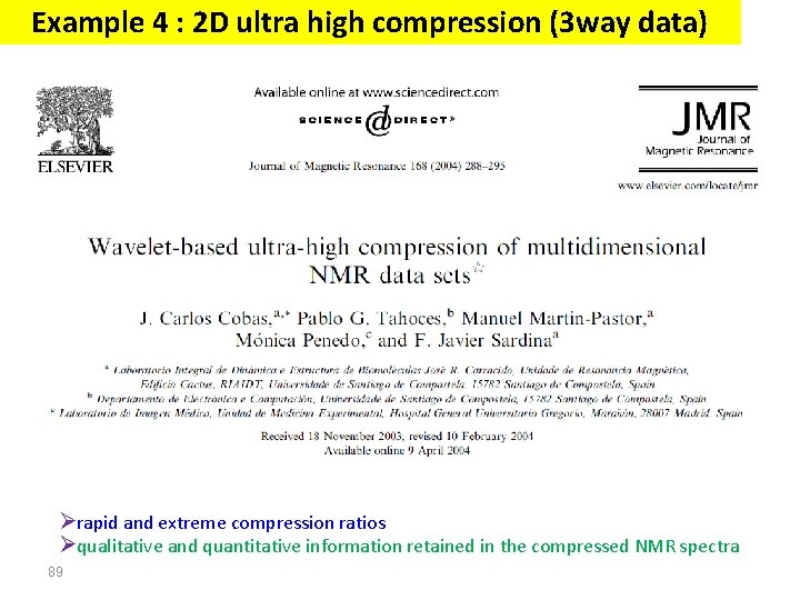
Example 4 : 2 D ultra high compression (3 way data) Ørapid and extreme compression ratios Øqualitative and quantitative information retained in the compressed NMR spectra 89

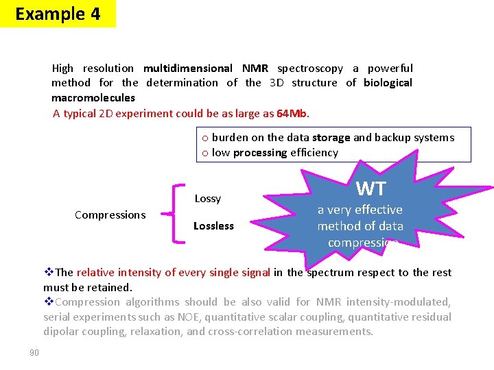
Example 4 High resolution multidimensional NMR spectroscopy a powerful method for the determination of the 3 D structure of biological macromolecules A typical 2 D experiment could be as large as 64 Mb. o burden on the data storage and backup systems o low processing efficiency Lossy Compressions Lossless WT a very effective method of data compression v. The relative intensity of every single signal in the spectrum respect to the rest must be retained. v. Compression algorithms should be also valid for NMR intensity-modulated, serial experiments such as NOE, quantitative scalar coupling, quantitative residual dipolar coupling, relaxation, and cross-correlation measurements. 90

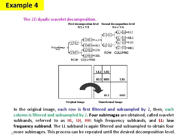
Example 4 The 2 D dyadic wavelet decomposition. In the original image, each row is first filtered and subsampled by 2, then, each column is filtered and subsampled by 2. Four subimages are obtained, called wavelet subbands, referred to as HL, LH, HH: high frequency subbands, and LL: low frequency subband. The LL subband is again filtered and subsampled to obtain four 91 more subimages. This process can be repeated until the desired decomposition level.

Example 4 Set partitioning in hierarchical trees (SPIHT) wavelet-based coding algorithm image compression 92

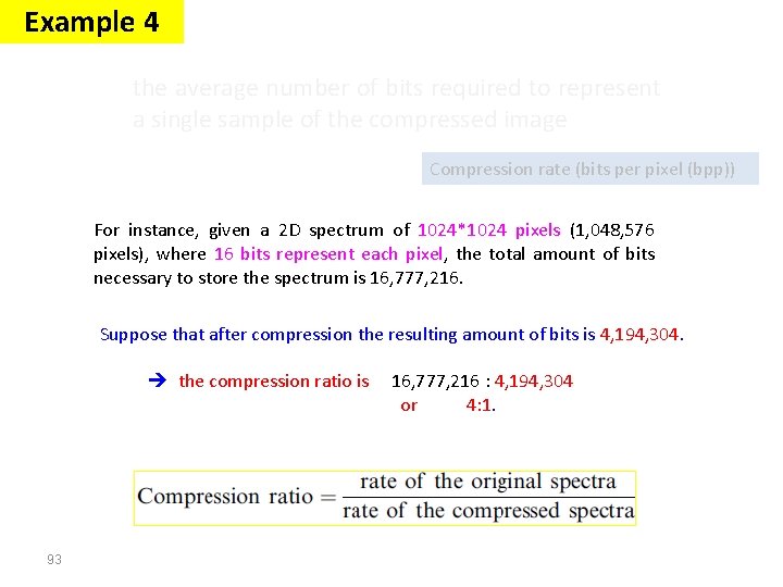
Example 4 the average number of bits required to represent a single sample of the compressed image Compression rate (bits per pixel (bpp)) For instance, given a 2 D spectrum of 1024*1024 pixels (1, 048, 576 pixels), where 16 bits represent each pixel, the total amount of bits necessary to store the spectrum is 16, 777, 216. Suppose that after compression the resulting amount of bits is 4, 194, 304. the compression ratio is 93 16, 777, 216 : 4, 194, 304 or 4: 1.

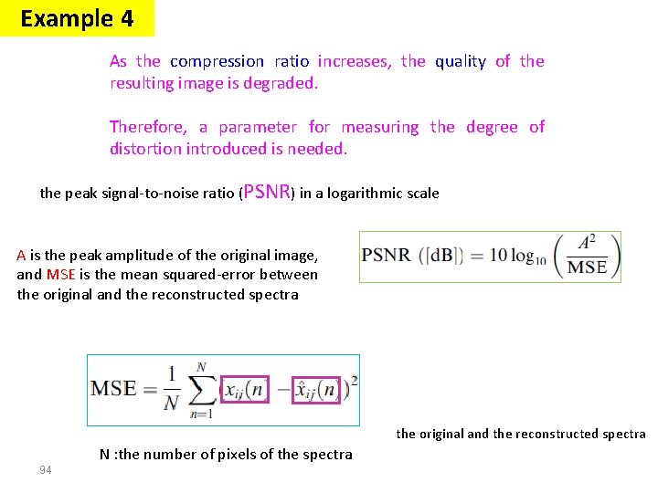
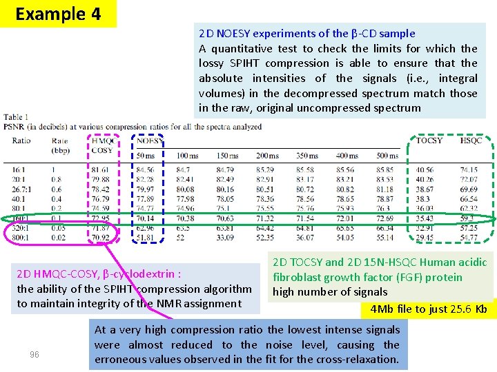
Example 4 As the compression ratio increases, the quality of the resulting image is degraded. Therefore, a parameter for measuring the degree of distortion introduced is needed. the peak signal-to-noise ratio (PSNR) in a logarithmic scale A is the peak amplitude of the original image, and MSE is the mean squared-error between the original and the reconstructed spectra N : the number of pixels of the spectra 94

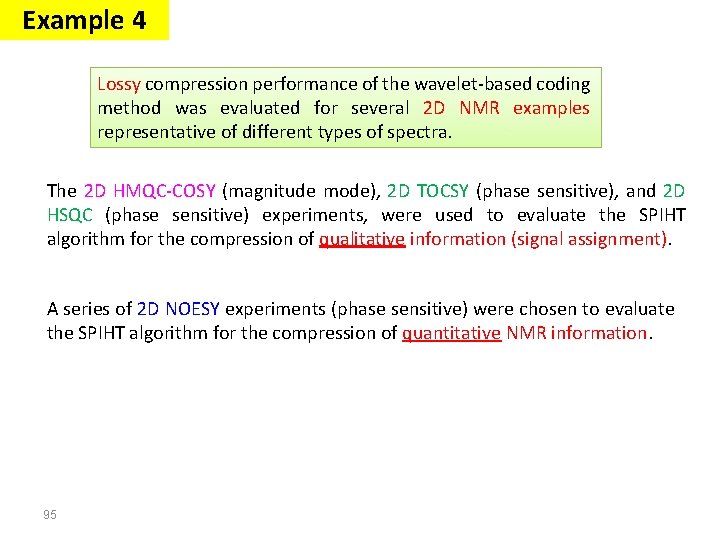
Example 4 Lossy compression performance of the wavelet-based coding method was evaluated for several 2 D NMR examples representative of different types of spectra. The 2 D HMQC-COSY (magnitude mode), 2 D TOCSY (phase sensitive), and 2 D HSQC (phase sensitive) experiments, were used to evaluate the SPIHT algorithm for the compression of qualitative information (signal assignment). A series of 2 D NOESY experiments (phase sensitive) were chosen to evaluate the SPIHT algorithm for the compression of quantitative NMR information. 95

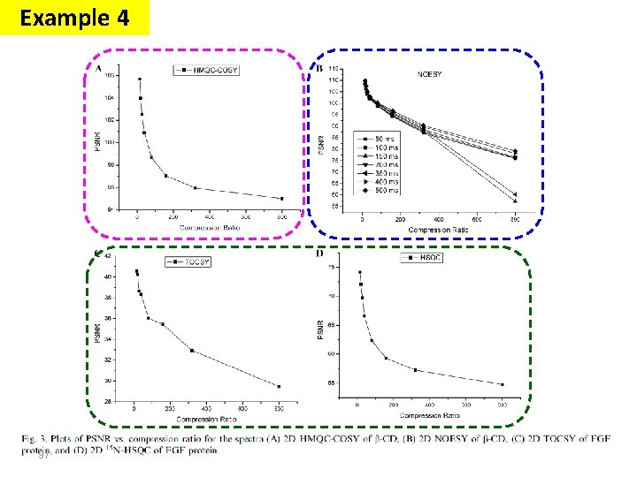
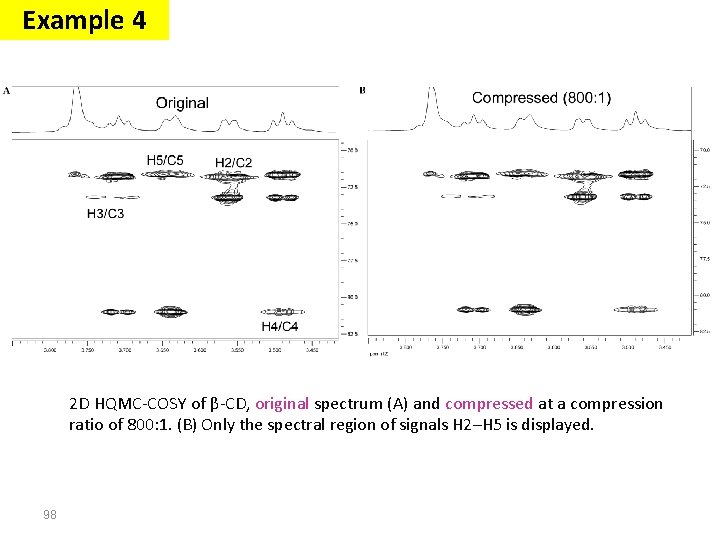
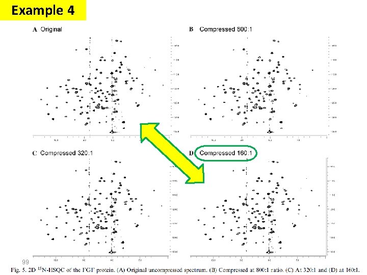
Example 4 2 D NOESY experiments of the β-CD sample A quantitative test to check the limits for which the lossy SPIHT compression is able to ensure that the absolute intensities of the signals (i. e. , integral volumes) in the decompressed spectrum match those in the raw, original uncompressed spectrum 2 D HMQC-COSY, β-cyclodextrin : the ability of the SPIHT compression algorithm to maintain integrity of the NMR assignment 96 2 D TOCSY and 2 D 15 N-HSQC Human acidic fibroblast growth factor (FGF) protein high number of signals 4 Mb file to just 25. 6 Kb At a very high compression ratio the lowest intense signals a loss of the least intense peaks were almost reduced to the noise level, causing the erroneous values observed in the fit for the cross-relaxation.

Example 4 97

Example 4 2 D HQMC-COSY of β-CD, original spectrum (A) and compressed at a compression ratio of 800: 1. (B) Only the spectral region of signals H 2–H 5 is displayed. 98

Example 4 99

Example 4 Conclusion High compression rates (up to 800: 1) can be achieved with the wavelet-based algorithm When the number of signals in the spectrum is not too high and the signal to noise ratio of the original spectrum is high, as it usually happens in HMQC and related experiments of medium-sized organic molecules, very high compression ratios can be used without risk of losing the qualitative chemical information. When quantitative information is required or the number of signals is high, more modest levels of compression should be used instead to avoid losing the information from the less intense peaks, but even in the most unfavorable cases, such as the quantification of small NOE intensities, a compression ratio of 80: 1 can be used safely. 100

Signal Processing The Fourier transform Stationary Signals Non-Stationary Signals Content : Short Time Fourier Analysis (or: Gabor Transform) Wavelet Transform Discrete Wavelet Transform Continuous Wavelet Transform Example 1 Example 2 Example 5 101

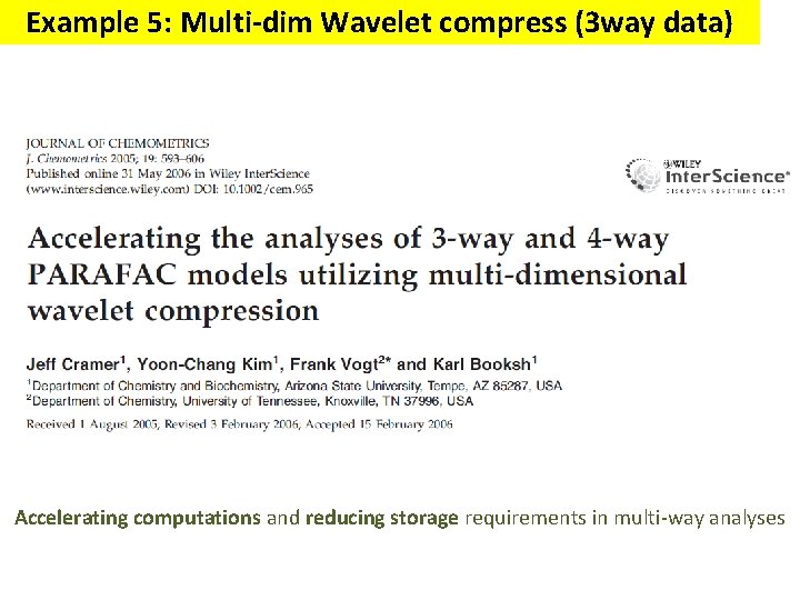
Example 5: Multi-dim Wavelet compress (3 way data) Accelerating computations and reducing storage requirements in multi-way analyses

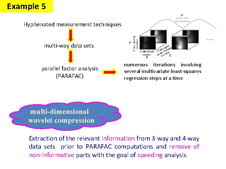
Example 5 Hyphenated measurement techniques multi-way data sets parallel factor analysis (PARAFAC) numerous iterations involving several multivariate least-squares regression steps at a time multi-dimensional wavelet compression Extraction of the relevant information from 3 -way and 4 -way data sets prior to PARAFAC computations and remove of non-informative parts with the goal of speeding analysis

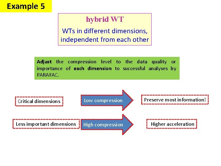
Example 5 hybrid WT WTs in different dimensions, independent from each other Adjust the compression level to the data quality or importance of each dimension to successful analyses by PARAFAC. Critical dimensions Less important dimensions Low compression High compression Preserve most information! Higher acceleration

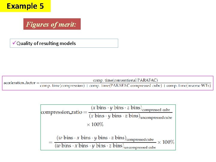
Example 5 Figures of merit: üQuality of resulting models

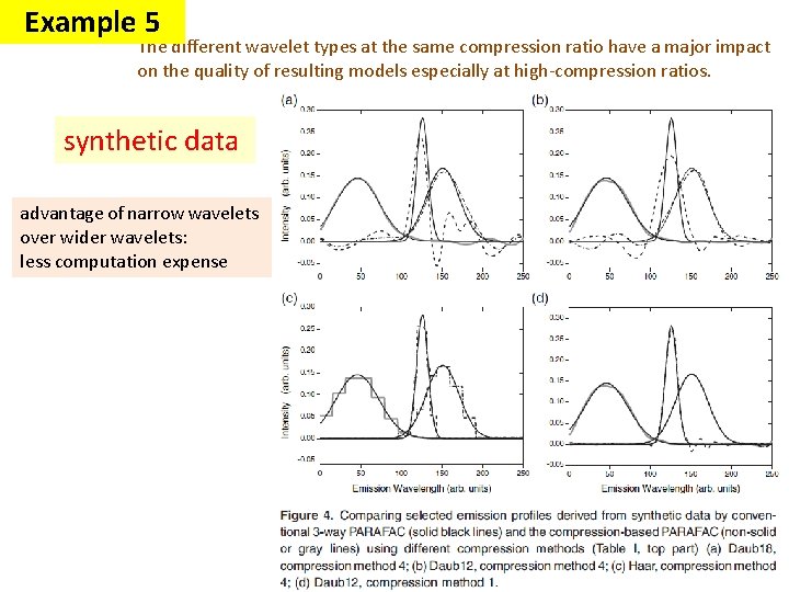
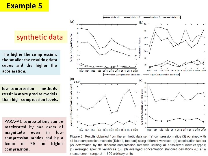
Example 5 The different wavelet types at the same compression ratio have a major impact on the quality of resulting models especially at high-compression ratios. synthetic data advantage of narrow wavelets over wider wavelets: less computation expense

Example 5 synthetic data The higher the compression, the smaller the resulting data cubes and the higher the acceleration. low-compression methods result in more precise models than high-compression levels. PARAFAC computations can be accelerated by one order of magnitude even in lowcompression modes and by a factor of 50 for higher compression.

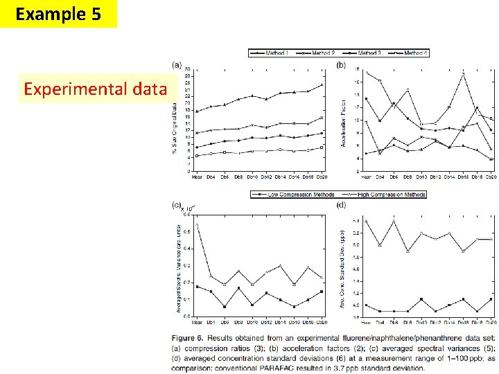
Example 5 Experimental data

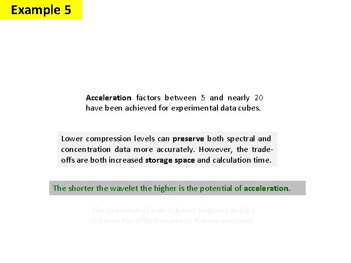
Example 5 Acceleration factors between 5 and nearly 20 have been achieved for experimental data cubes. Lower compression levels can preserve both spectral and concentration data more accurately. However, the tradeoffs are both increased storage space and calculation time. The shorter the wavelet the higher is the potential of acceleration. The presence of non-trilinear features in data reduces the effectiveness of the compression.

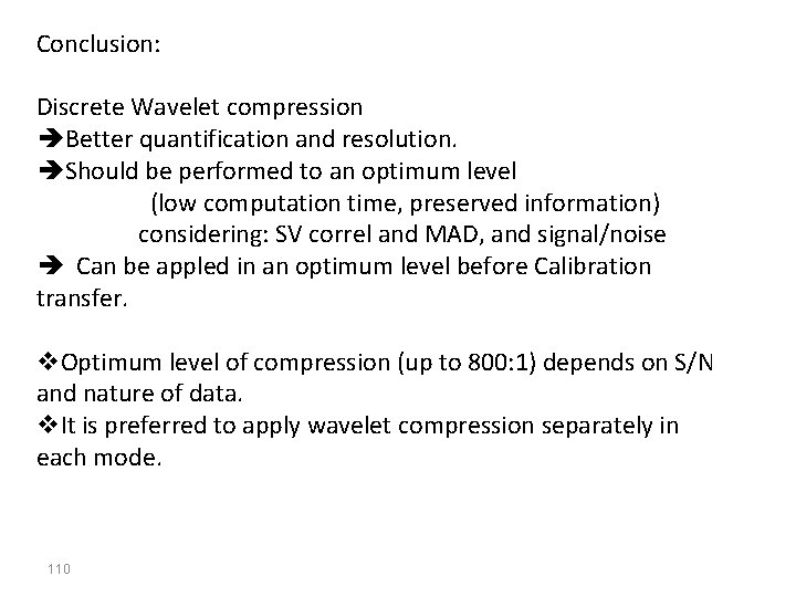
Conclusion: Discrete Wavelet compression Better quantification and resolution. Should be performed to an optimum level (low computation time, preserved information) considering: SV correl and MAD, and signal/noise Can be appled in an optimum level before Calibration transfer. v. Optimum level of compression (up to 800: 1) depends on S/N and nature of data. v. It is preferred to apply wavelet compression separately in each mode. 110

111 Thanks for your attention