Datalog and Emerging Applications an Interactive Tutorial Shan

Datalog and Emerging Applications: an Interactive Tutorial Shan Huang T. J. Green Boon Thau Loo SIGMOD 2011 Athens, Greece June 14, 2011

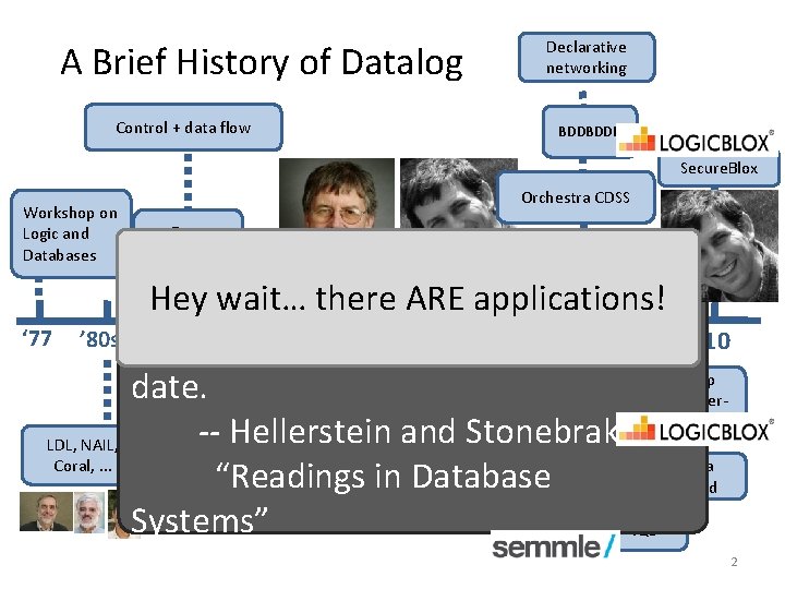
A Brief History of Datalog Control + data flow Declarative networking BDDBDDB Secure. Blox Workshop on Logic and Databases Orchestra CDSS Data integration Information Extraction No practical applications of recursive Hey wait… there ARE applications! ‘ 77 ’ 80 s …query ‘ 95 theory … have been ‘ 05 ‘ 07 ‘ 02 found to‘ 08 ‘ 10 Doop date. (pointeranalysis) Access control -- Hellerstein and Stonebraker LDL, NAIL, (Binder) Coral, . . . Evita “Readings in Database Raced Systems”. QL 2

Today’s Tutorial, or, Datalog: Taste it Again for the First Time • We review the basics and examine several of these recent applications • Theme #1: lots of compelling applications, if we look beyond payroll / bill-of-materials /. . . – Some of the most interesting work coming from outside databases community! • Theme #2: language extensions usually needed – To go from a toy language to something really usable 3

) ! y l s u o n o (Asynchr An Interactive Tutorial ^ INSTALL_LB : installation guide README : structure of distribution files Quick-Start guide : usage *. logic : Datalog examples *. lb : Logic. Blox interactive shell script (to drive the Datalog examples) • Shan and other Logic. Blox folks will be available immediately after talk for the “synchronous” version of tutorial • • • 4

Outline of Tutorial June 14, 2011: The Second Coming of Datalog! • • • Refresher: Datalog 101 Application #1: Data Integration and Exchange Application #2: Program Analysis Application #3: Declarative Networking Conclusions 5

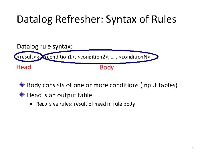
Datalog Refresher: Syntax of Rules Datalog rule syntax: <result> <condition 1>, <condition 2>, … , <condition. N>. Head Body consists of one or more conditions (input tables) Head is an output table n Recursive rules: result of head in rule body 6

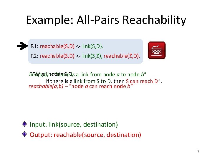
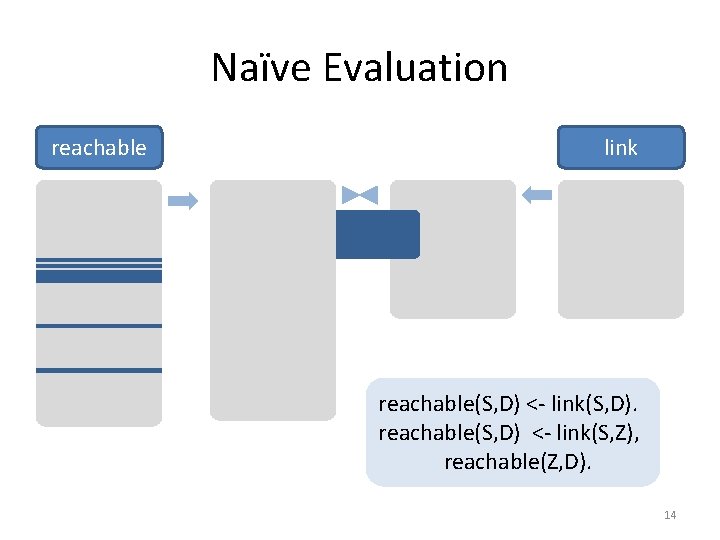
Example: All-Pairs Reachability R 1: reachable(S, D) <- link(S, D). R 2: reachable(S, D) <- link(S, Z), reachable(Z, D). “For all nodes S, D, is a link from node a to node b” link(a, b) – “there If there is a link from S to D, then S can reach D”. reachable(a, b) – “node a can reach node b” Input: link(source, destination) Output: reachable(source, destination) 7

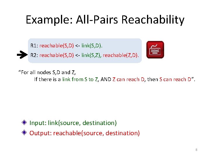
Example: All-Pairs Reachability R 1: reachable(S, D) <- link(S, D). R 2: reachable(S, D) <- link(S, Z), reachable(Z, D). “For all nodes S, D and Z, If there is a link from S to Z, AND Z can reach D, then S can reach D”. Input: link(source, destination) Output: reachable(source, destination) 8

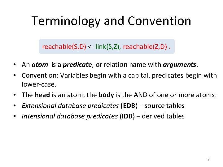
Terminology and Convention reachable(S, D) <- link(S, Z), reachable(Z, D). • An atom is a predicate, or relation name with arguments. • Convention: Variables begin with a capital, predicates begin with lower-case. • The head is an atom; the body is the AND of one or more atoms. • Extensional database predicates (EDB) – source tables • Intensional database predicates (IDB) – derived tables 9

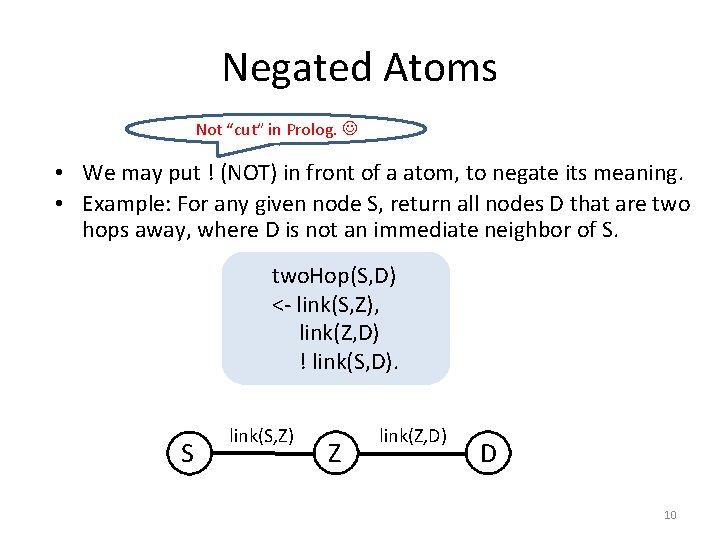
Negated Atoms Not “cut” in Prolog. • We may put ! (NOT) in front of a atom, to negate its meaning. • Example: For any given node S, return all nodes D that are two hops away, where D is not an immediate neighbor of S. two. Hop(S, D) <- link(S, Z), link(Z, D) ! link(S, D). S link(S, Z) Z link(Z, D) D 10

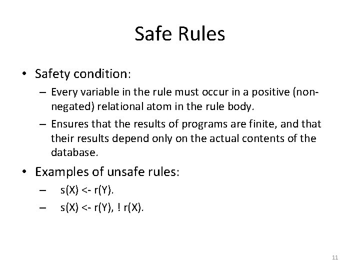
Safe Rules • Safety condition: – Every variable in the rule must occur in a positive (nonnegated) relational atom in the rule body. – Ensures that the results of programs are finite, and that their results depend only on the actual contents of the database. • Examples of unsafe rules: – – s(X) <- r(Y), ! r(X). 11

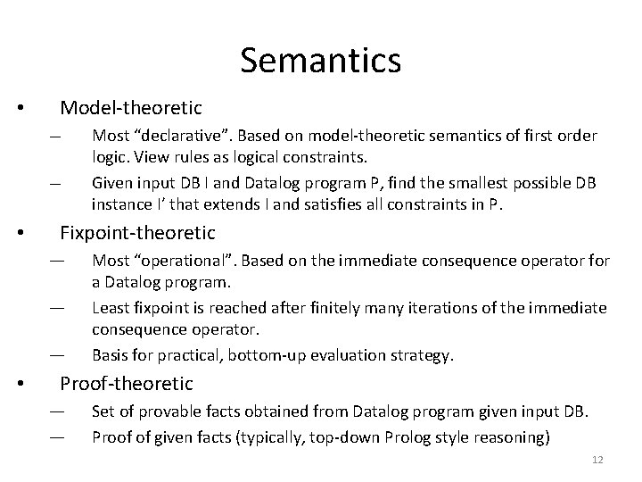
Semantics • Model-theoretic — — • Fixpoint-theoretic — — — • Most “declarative”. Based on model-theoretic semantics of first order logic. View rules as logical constraints. Given input DB I and Datalog program P, find the smallest possible DB instance I’ that extends I and satisfies all constraints in P. Most “operational”. Based on the immediate consequence operator for a Datalog program. Least fixpoint is reached after finitely many iterations of the immediate consequence operator. Basis for practical, bottom-up evaluation strategy. Proof-theoretic — — Set of provable facts obtained from Datalog program given input DB. Proof of given facts (typically, top-down Prolog style reasoning) 12

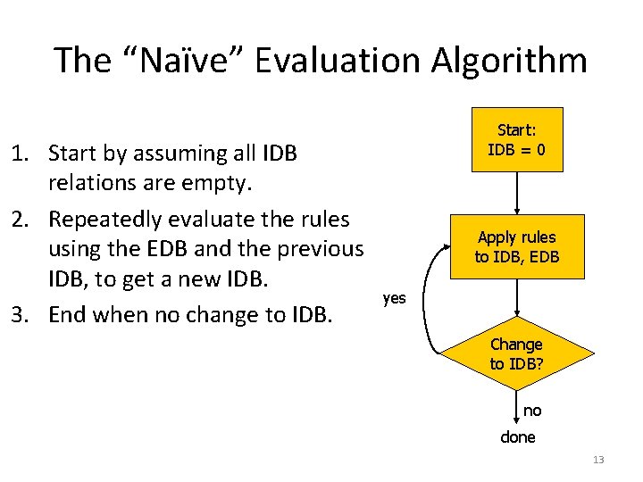
The “Naïve” Evaluation Algorithm 1. Start by assuming all IDB relations are empty. 2. Repeatedly evaluate the rules using the EDB and the previous IDB, to get a new IDB. 3. End when no change to IDB. Start: IDB = 0 Apply rules to IDB, EDB yes Change to IDB? no done 13

Naïve Evaluation reachable link reachable(S, D) <- link(S, D). reachable(S, D) <- link(S, Z), reachable(Z, D). 14

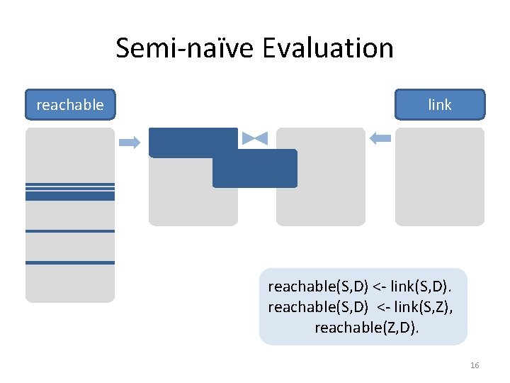
Semi-naïve Evaluation • Since the EDB never changes, on each round we only get new IDB tuples if we use at least one IDB tuple that was obtained on the previous round. • Saves work; lets us avoid rediscovering most known facts. – A fact could still be derived in a second way. 15

Semi-naïve Evaluation reachable link reachable(S, D) <- link(S, D). reachable(S, D) <- link(S, Z), reachable(Z, D). 16

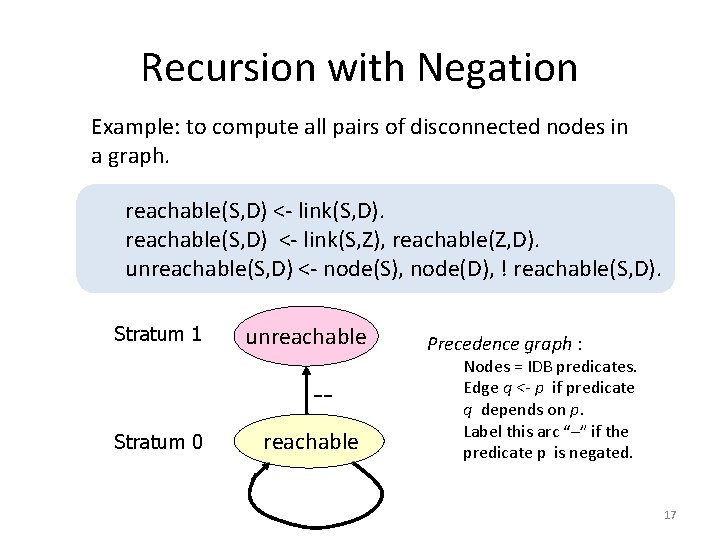
Recursion with Negation Example: to compute all pairs of disconnected nodes in a graph. reachable(S, D) <- link(S, D). reachable(S, D) <- link(S, Z), reachable(Z, D). unreachable(S, D) <- node(S), node(D), ! reachable(S, D). Stratum 1 unreachable -Stratum 0 reachable Precedence graph : Nodes = IDB predicates. Edge q <- p if predicate q depends on p. Label this arc “–” if the predicate p is negated. 17

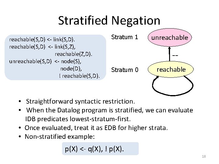
Stratified Negation reachable(S, D) <- link(S, D). reachable(S, D) <- link(S, Z), reachable(Z, D). unreachable(S, D) <- node(S), node(D), ! reachable(S, D). Stratum 1 unreachable -Stratum 0 reachable • Straightforward syntactic restriction. • When the Datalog program is stratified, we can evaluate IDB predicates lowest-stratum-first. • Once evaluated, treat it as EDB for higher strata. • Non-stratified example: p(X) <- q(X), ! p(X). 18

A Sneak Preview… • Data integration – Skolem functions • Program analysis – Type-based optimization • Declarative networking – Aggregates, aggregate selections – Incremental view maintenance – Magic sets 19

Suggested Readings • Survey papers: • A Survey of Research on Deductive Database Systems, Ramakrishnan and Ullman, Journal of Logic Programming, 1993 • What you always wanted to know about datalog (and never dared to ask), by Ceri, Gottlob, and Tanca. • An Amateur’s Expert’s Guide to Recursive Query Processing, Bancilhon and Ramakrishnan, SIGMOD Record. • Database Encyclopedia entry on “DATALOG”. Grigoris Karvounarakis. • Textbooks: • • Foundations in Databases. Abiteboul, Hull, Vianu. Database Management Systems, Ramakrishnan and Gehkre. Chapter on “Deductive Databases”. • Acknowledgements: • • Jeff Ullman’s CIS 145 class lecture slides. Raghu Ramakrishnan and Johannes Gehrke’s lecture slides for Database Management Systems textbook. 20

Outline of Tutorial June 14, 2011: The Second Coming of Datalog! • • • Refresher: Datalog 101 Application #1: Data Integration and Exchange Application #2: Program Analysis Application #3: Declarative Networking Conclusions 21

Datalog for Data Integration • Motivation and problem setting • Two basic approaches: – virtual data integration – materialized data exchange • Schema mappings and Datalog with Skolem functions 22

The Data Integration Problem • Have a collection of related data sources with – different schemas – different data models (relational, XML, plain text, . . . ) – different attribute domains – different capabilities / availability • Need to cobble them together and provide a uniform interface • Want to keep track of what came from where • Focus here: solving problem of different schemas (schema heterogeneity) for relational data 23

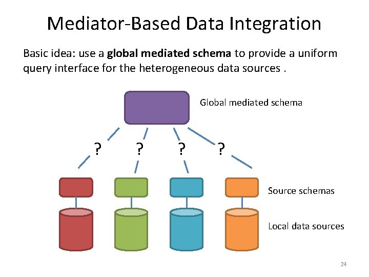
Mediator-Based Data Integration Basic idea: use a global mediated schema to provide a uniform query interface for the heterogeneous data sources. Global mediated schema ? ? Source schemas Local data sources 24

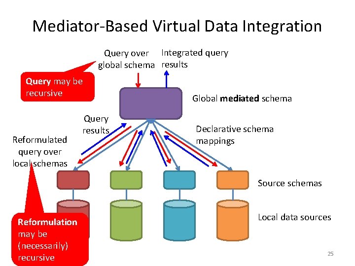
Mediator-Based Virtual Data Integration Query over Integrated query global schema results Query may be recursive Reformulated query over local schemas Query results Global mediated schema Declarative schema mappings Source schemas Reformulation may be (necessarily) recursive Local data sources 25

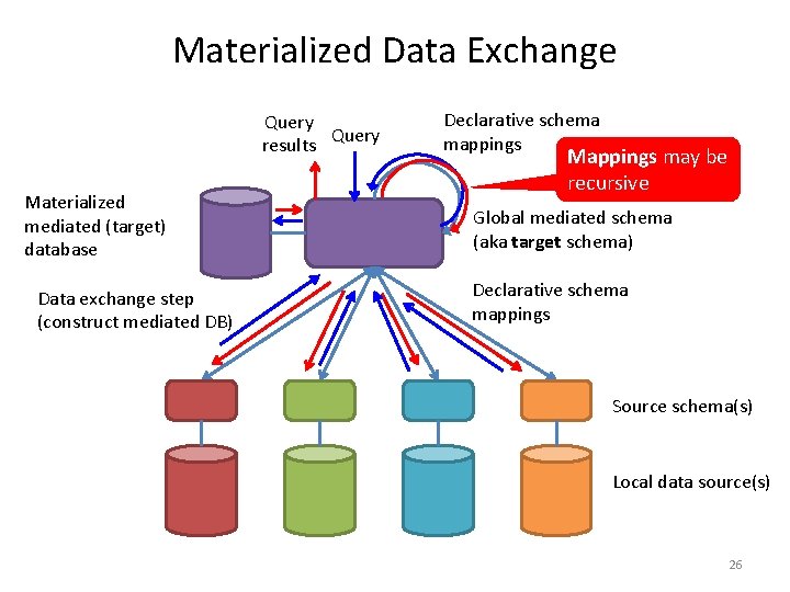
Materialized Data Exchange Query results Materialized mediated (target) database Data exchange step (construct mediated DB) Declarative schema mappings Mappings may be recursive Global mediated schema (aka target schema) Declarative schema mappings Source schema(s) Local data source(s) 26

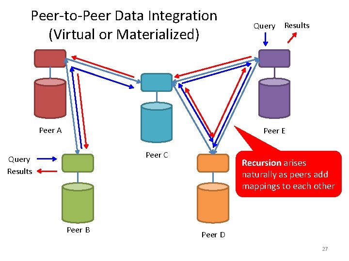
Peer-to-Peer Data Integration (Virtual or Materialized) Peer A Query Results Peer E Peer C Query Results Peer B Recursion arises naturally as peers add mappings to each other Peer D 27

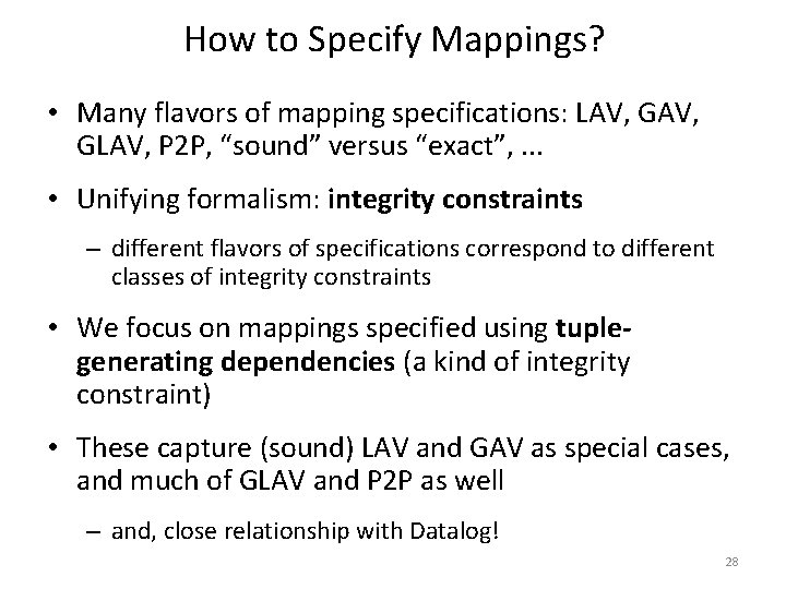
How to Specify Mappings? • Many flavors of mapping specifications: LAV, GLAV, P 2 P, “sound” versus “exact”, . . . • Unifying formalism: integrity constraints – different flavors of specifications correspond to different classes of integrity constraints • We focus on mappings specified using tuplegenerating dependencies (a kind of integrity constraint) • These capture (sound) LAV and GAV as special cases, and much of GLAV and P 2 P as well – and, close relationship with Datalog! 28

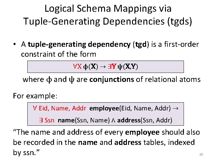
Logical Schema Mappings via Tuple-Generating Dependencies (tgds) • A tuple-generating dependency (tgd) is a first-order constraint of the form ∀X ϕ(X) → ∃Y ψ(X, Y) where ϕ and ψ are conjunctions of relational atoms For example: ∀ Eid, Name, Addr employee(Eid, Name, Addr) → ∃ Ssn name(Ssn, Name) ∧ address(Ssn, Addr) “The name and address of every employee should also be recorded in the name and address tables, indexed by ssn. ” 29

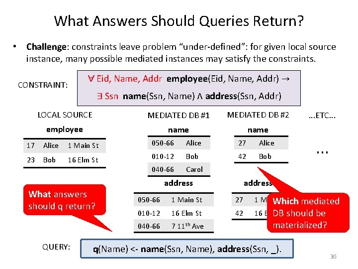
What Answers Should Queries Return? • Challenge: constraints leave problem “under-defined”: for given local source instance, many possible mediated instances may satisfy the constraints. ∀ Eid, Name, Addr employee(Eid, Name, Addr) → CONSTRAINT: 17 23 ∃ Ssn name(Ssn, Name) ∧ address(Ssn, Addr) LOCAL SOURCE MEDIATED DB #1 MEDIATED DB #2 employee name Alice Bob 1 Main St 050 -66 Alice 27 Alice 16 Elm St 010 -12 Bob 42 Bob 040 -66 Carol What answers should q return? QUERY: address 050 -66 1 Main St 27 010 -12 16 Elm St 42 040 -66 7 11 th Ave . . . ETC. . 1 Main St Which mediated 16 Elm St should be DB materialized? q(Name) <- name(Ssn, Name), address(Ssn, _). 30

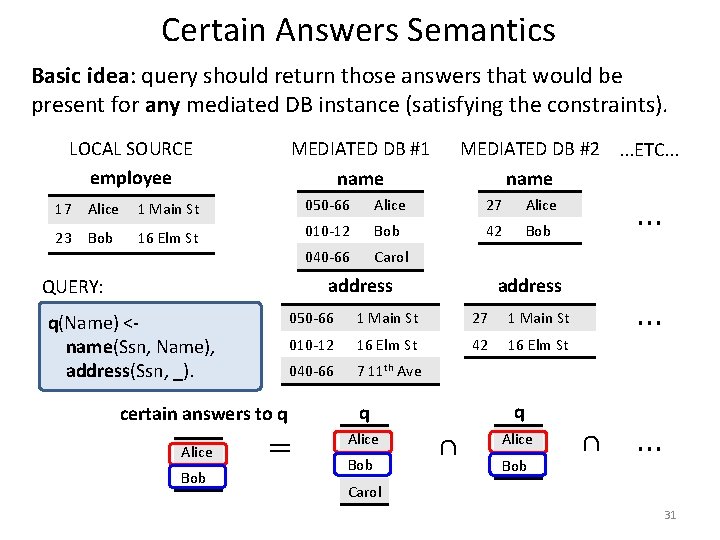
Certain Answers Semantics Basic idea: query should return those answers that would be present for any mediated DB instance (satisfying the constraints). MEDIATED DB #1 name LOCAL SOURCE employee 17 23 Alice Bob MEDIATED DB #2. . . ETC. . . name 1 Main St 050 -66 Alice 27 Alice 16 Elm St 010 -12 Bob 42 Bob 040 -66 Carol address QUERY: q(Name) <name(Ssn, Name), address(Ssn, _). Alice Bob address 050 -66 1 Main St 27 1 Main St 010 -12 16 Elm St 42 16 Elm St 040 -66 7 11 th Ave certain answers to q = q q Alice Bob . . . ∩ Alice Bob . . . ∩ . . . Carol 31

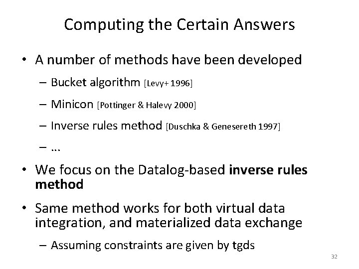
Computing the Certain Answers • A number of methods have been developed – Bucket algorithm [Levy+ 1996] – Minicon [Pottinger & Halevy 2000] – Inverse rules method [Duschka & Genesereth 1997] –. . . • We focus on the Datalog-based inverse rules method • Same method works for both virtual data integration, and materialized data exchange – Assuming constraints are given by tgds 32

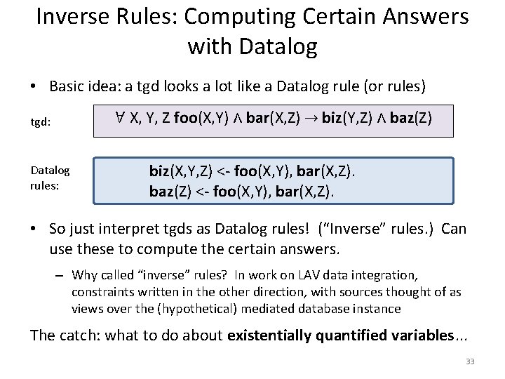
Inverse Rules: Computing Certain Answers with Datalog • Basic idea: a tgd looks a lot like a Datalog rule (or rules) ∀ X, Y, Z foo(X, Y) ∧ bar(X, Z) → biz(Y, Z) ∧ baz(Z) tgd: Datalog rules: biz(X, Y, Z) <- foo(X, Y), bar(X, Z). baz(Z) <- foo(X, Y), bar(X, Z). • So just interpret tgds as Datalog rules! (“Inverse” rules. ) Can use these to compute the certain answers. – Why called “inverse” rules? In work on LAV data integration, constraints written in the other direction, with sources thought of as views over the (hypothetical) mediated database instance The catch: what to do about existentially quantified variables. . . 33

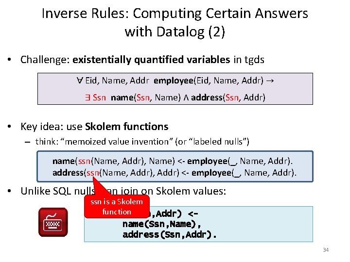
Inverse Rules: Computing Certain Answers with Datalog (2) • Challenge: existentially quantified variables in tgds ∀ Eid, Name, Addr employee(Eid, Name, Addr) → ∃ Ssn name(Ssn, Name) ∧ address(Ssn, Addr) • Key idea: use Skolem functions – think: “memoized value invention” (or “labeled nulls”) name(ssn(Name, Addr), Name) <- employee(_, Name, Addr). address(ssn(Name, Addr) <- employee(_, Name, Addr). • Unlike SQL nulls, can join on Skolem values: ssn is a Skolem function query _(Name, Addr) <name(Ssn, Name), address(Ssn, Addr). 34

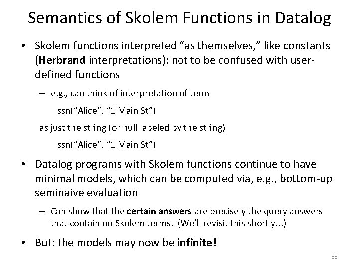
Semantics of Skolem Functions in Datalog • Skolem functions interpreted “as themselves, ” like constants (Herbrand interpretations): not to be confused with userdefined functions – e. g. , can think of interpretation of term ssn(“Alice”, “ 1 Main St”) as just the string (or null labeled by the string) ssn(“Alice”, “ 1 Main St”) • Datalog programs with Skolem functions continue to have minimal models, which can be computed via, e. g. , bottom-up seminaive evaluation – Can show that the certain answers are precisely the query answers that contain no Skolem terms. (We’ll revisit this shortly. . . ) • But: the models may now be infinite! 35

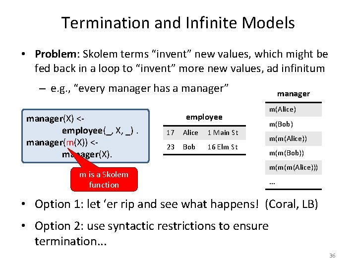
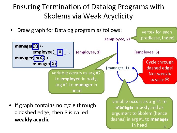
Termination and Infinite Models • Problem: Skolem terms “invent” new values, which might be fed back in a loop to “invent” more new values, ad infinitum – e. g. , “every manager has a manager” manager(X) <employee(_, X, _). manager(m(X)) <manager(X). employee 17 Alice 1 Main St 23 Bob 16 Elm St m is a Skolem function manager m(Alice) m(Bob) m(m(Alice)) m(m(Bob)) m(m(m(Alice))). . . • Option 1: let ‘er rip and see what happens! (Coral, LB) • Option 2: use syntactic restrictions to ensure termination. . . 36

Ensuring Termination of Datalog Programs with Skolems via Weak Acyclicity • Draw graph for Datalog program as follows: (employee, 2) manager(X) <employee(_, X, _). manager(m(X)) <manager(X). (employee, 1) variable occurs as arg #2 to employee in body, arg #1 to manager in head • If graph contains no cycle through a dashed edge, then P is called weakly acyclic vertex for each (predicate, index) (employee, 3) (manager, 1) Cycle through dashed edge! Not weakly acyclic variable occurs as arg #1 to manager in body and as argument to Skolem (hence dashes) in arg #1 to manager in head 37

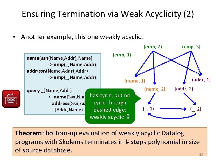
Ensuring Termination via Weak Acyclicity (2) • Another example, this one weakly acyclic: (emp, 2) name(ssn(Name, Addr), Name) <- emp(_, Name, Addr). addr(ssn(Name, Addr) <- emp(_, Name, Addr). (emp, 3) (emp, 1) (name, 1) query _(Name, Addr) has cycle, but no <- name(Ssn, Name), address(Ssn, Addr) ; cycle through _(Addr, Name). dashed edge; (name, 2) (_, 1) (addr, 2) (_, 2) weakly acyclic Theorem: bottom-up evaluation of weakly acyclic Datalog programs with Skolems terminates in # steps polynomial in size of source database. 38

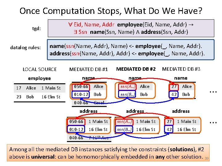
Once Computation Stops, What Do We Have? ∀ Eid, Name, Addr employee(Eid, Name, Addr) → ∃ Ssn name(Ssn, Name) ∧ address(Ssn, Addr) tgd: datalog rules: 17 23 name(ssn(Name, Addr), Name) <- employee(_, Name, Addr). address(ssn(Name, Addr) <- employee(_, Name, Addr). LOCAL SOURCE MEDIATED DB #1 MEDIATED DB #2 MEDIATED DB #3 employee name Alice Bob 1 Main St 16 Elm St 050 -66 Alice ssn(A. . ) Alice 27 Alice 010 -12 Bob ssn(B. . ) Bob 42 Bob 040 -66 Carol address 050 -66 1 Main St ssn(A. . ) 1 Main St 27 1 Main St 010 -12 16 Elm St ssn(B. . ) 16 Elm St 42 16 Elm St 040 -66 7 11 th Ave Among all the mediated DB instances satisfying the constraints (solutions), #2 above is universal: can be homomorphically embedded in any other solution. 39 . . .

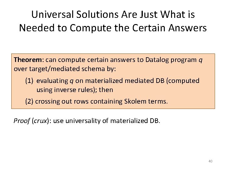
Universal Solutions Are Just What is Needed to Compute the Certain Answers Theorem: can compute certain answers to Datalog program q over target/mediated schema by: (1) evaluating q on materialized mediated DB (computed using inverse rules); then (2) crossing out rows containing Skolem terms. Proof (crux): use universality of materialized DB. 40

Notes on Skolem Functions in Datalog • Notion of weak acyclicity introduced by Deutsch and Popa, as a way to ensure termination of the chase procedure for logical dependencies (but applies to Datalog too). • Crazy idea: what if we allow arbitrary use of Skolems, and forget about computing complete output idb’s bottom-up, but only partially enumerate their contents, on demand, using top-down evaluation? – And, while we’re at it, allow unsafe rules too? • This is actually a beautiful idea: it’s called logic programming – Skolem functions (aka “functor terms”) are how you build data structures like lists, trees, etc. in Prolog – Resulting language is Turing-complete 41

Summary: Datalog for Data Integration and Exchange • Datalog serves as very nice language for schema mappings, as needed in data integration, provided we extend it with Skolem functions – Can use Datalog to compute certain answers – Fancier kinds of schema mappings than tgds require further language extensions; e. g. , Datalog +/- [Cali et al 09] • Can also extend Datalog to track various kinds of data provenance, very useful in data integration – Using semiring-based framework [Green+ 07] 42

Some Datalog-Based Data Integration/Exchange Systems • Information Manifold [Levy+ 96] – Virtual approach – No recursion • Clio [Miller+ 01] – Materialized approach – Skolem terms, no recursion, rich data model – Ships as part of IBM Web. Sphere • Orchestra CDSS [Ives+ 05] – Materialized approach – Skolem terms, recursion, provenance, updates 43

Datalog for Data Integration: Some Open Issues • Materialized data exchange: renewed need for efficient incremental view maintenance algorithms – Source databases are dynamic entities, need to propagate changes – Classical algorithm DRed [Gupta+ 93] often performs very badly; newer provenance-based algorithms [Green+ 07, Liu+ 08] faster but incur space overhead; can we do better? • Termination for Datalog with Skolems – Improvements on weak ayclicity for chase termination, translate to Datalog; more permissive conditions always useful! – Is termination even decidable? (Undecidable if we allow Skolems and unsafe rules, of course. ) 44

Outline of Tutorial June 14, 2011: The Second Coming of Datalog! • • • Refresher: basics of Datalog Application #1: Data Integration and Exchange Application #2: Program Analysis Application #3: Declarative Networking Conclusion 45

Program Analysis • What is it? – Fundamental analysis aiding software development – Help make programs run fast, help you find bugs • Why in Datalog? – Declarative recursion • How does it work? – Really well! An order-of-magnitude faster than handtuned, Java tools – Datalog optimizations are crucial in achieving performance 46

WHAT IS PROGRAM ANALYSIS 47

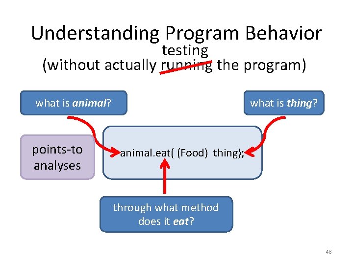
Understanding Program Behavior testing (without actually running the program) what is animal? points-to analyses what is thing? animal. eat( (Food) thing); through what method does it eat? 48

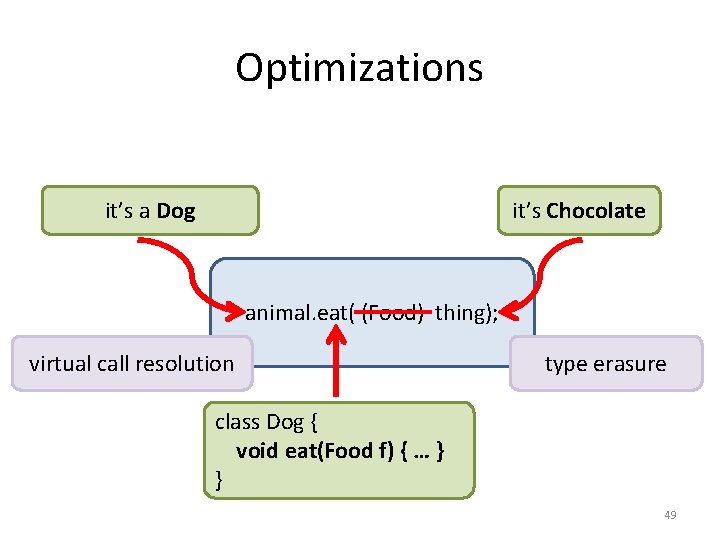
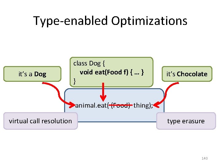
Optimizations what it’sisaanimal? Dog what it’s Chocolate is thing? animal. eat( (Food) thing); virtual call resolution type erasure class Dog {what method through void does eat(Food f) { … } it eat? } 49

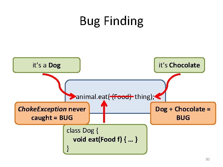
Bug Finding what it’sisaanimal? Dog what it’s Chocolate is thing? animal. eat( (Food) thing); Choke. Exception never caught = BUG Dog + Chocolate = BUG class Dog {what method through void does eat(Food f) { … } it eat? } 50

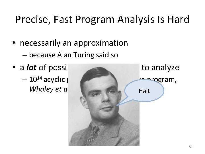
Precise, Fast Program Analysis Is Hard • necessarily an approximation – because Alan Turing said so • a lot of possible execution paths to analyze – 1014 acyclic paths in an average Java program, Whaley et al. , ‘ 05 Halt 51

WHY PROGRAM ANALYSIS IN DATALOG? 52

WHY PROGRAM ANALYSIS IN A DECLARATIVE LANGUAGE? WHY DATALOG? 53

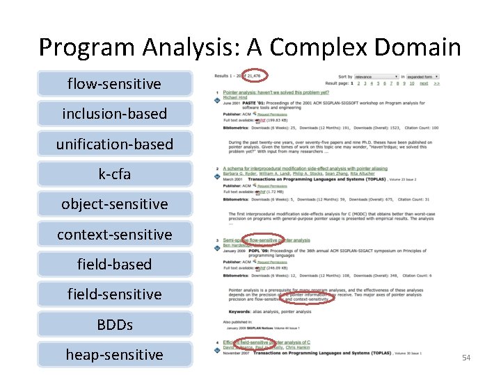
Program Analysis: A Complex Domain flow-sensitive inclusion-based unification-based k-cfa object-sensitive context-sensitive field-based field-sensitive BDDs heap-sensitive 54

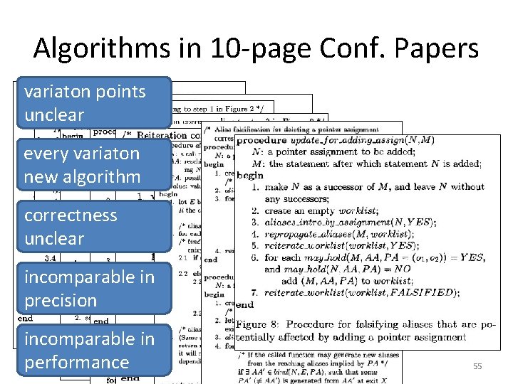
Algorithms in 10 -page Conf. Papers variaton points unclear every variaton new algorithm correctness unclear incomparable in precision incomparable in performance 55

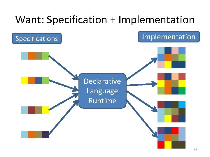
Want: Specification + Implementation Specifications Declarative Language Runtime 56

DECLARATIVE = GOOD WHY DATALOG? 57

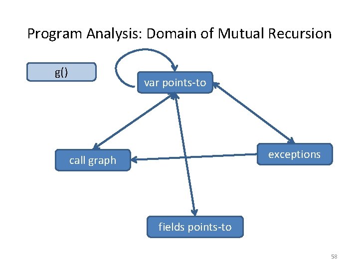
Program Analysis: Domain of Mutual Recursion catch xthrow xxx. f ===g() y. f(); =y. f; y; (Ey; ee) var points-to exceptions call graph fields points-to 58

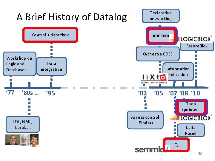
A Brief History of Datalog Control + data flow Declarative networking BDDBDDB Secure. Blox Workshop on Logic and Databases ‘ 77 ’ 80 s … LDL, NAIL, Coral, . . . Orchestra CDSS Data integration ‘ 95 Information Extraction ‘ 02 ‘ 05 ‘ 07 ‘ 08 ‘ 10 Doop (pointeranalysis) Access control (Binder) Evita Raced. QL 59

PROGRAM ANALYSIS IN DATALOG 60

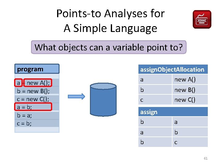
Points-to Analyses for A Simple Language What objects can a variable point to? program a = new A(); b = new B(); c = new C(); a = b; b = a; c = b; assign. Object. Allocation a new A() b c new B() new C() assign b a a b b c 61

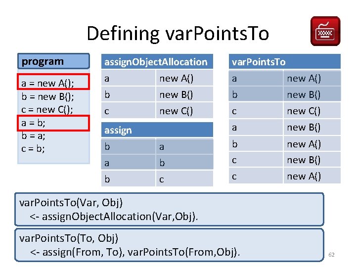
Defining var. Points. To program a = new A(); b = new B(); c = new C(); a = b; b = a; c = b; assign. Object. Allocation a new A() var. Points. To a new A() b c new B() new C() a new B() b c c new A() new B() new C() assign b a a b b c var. Points. To(Var, Obj) <- assign. Object. Allocation(Var, Obj). var. Points. To(To, Obj) <- assign(From, To), var. Points. To(From, Obj). 62

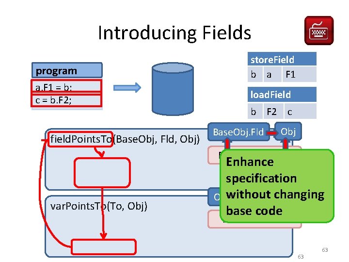
Introducing Fields program a. F 1 = b; c = b. F 2; store. Field b a F 1 load. Field b F 2 c Base. Obj. Fld Obj field. Points. To(Base. Obj, Fld, Obj) <- store. Field(From, Base, Fld), Base. Fld = From Enhance var. Points. To(Base, Base. Obj), specification var. Points. To(From, Obj). changing Objwithout Base. Obj. Fld var. Points. To(To, Obj) base code To = Base. Fld <- load. Field(Base, Fld, To), var. Points. To(Base, Base. Obj), field. Points. To(Base. Obj, Fld, Obj). 63 63

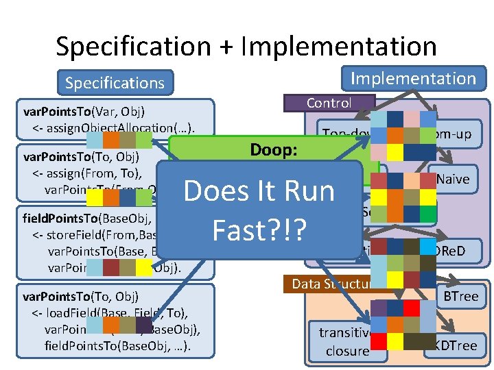
Specification + Implementation Specifications Control var. Points. To(Var, Obj) <- assign. Object. Allocation(…). var. Points. To(To, Obj) <- assign(From, To), var. Points. To(From, Obj). Top-down Doop: ~2500 lines of logic Tabled Bottom-up Naive Does It Run Datalog Semi-naive field. Points. To(Base. Obj, Fld, Obj) Engine <- store. Field(From, Base, Field), Fast? !? var. Points. To(Base, Base. Obj), Counting DRe. D var. Points. To(From, Obj). var. Points. To(To, Obj) <- load. Field(Base, Field, To), var. Points. To(Base, Base. Obj), field. Points. To(Base. Obj, …). Data Structures BDDs transitive closure BTree KDTree 64

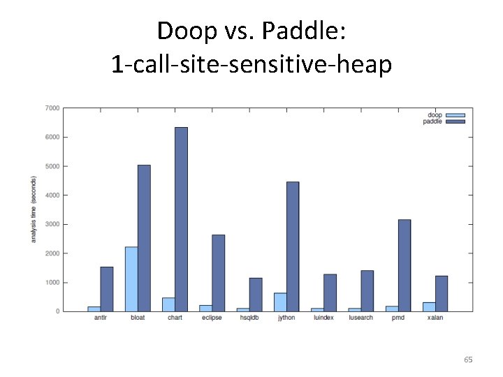
Doop vs. Paddle: 1 -call-site-sensitive-heap 65

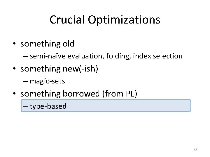
Crucial Optimizations • something old – semi-naïve evaluation, folding, index selection • something new(-ish) – magic-sets • something borrowed (from PL) – type-based 66

TYPE-BASED OPTIMIZATIONS 67

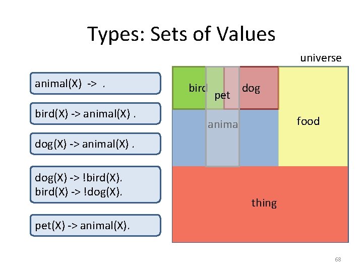
Types: Sets of Values universe animal(X) ->. bird(X) -> animal(X). bird pet dog food animal dog(X) -> animal(X). dog(X) -> !bird(X) -> !dog(X). thing pet(X) -> animal(X). 68

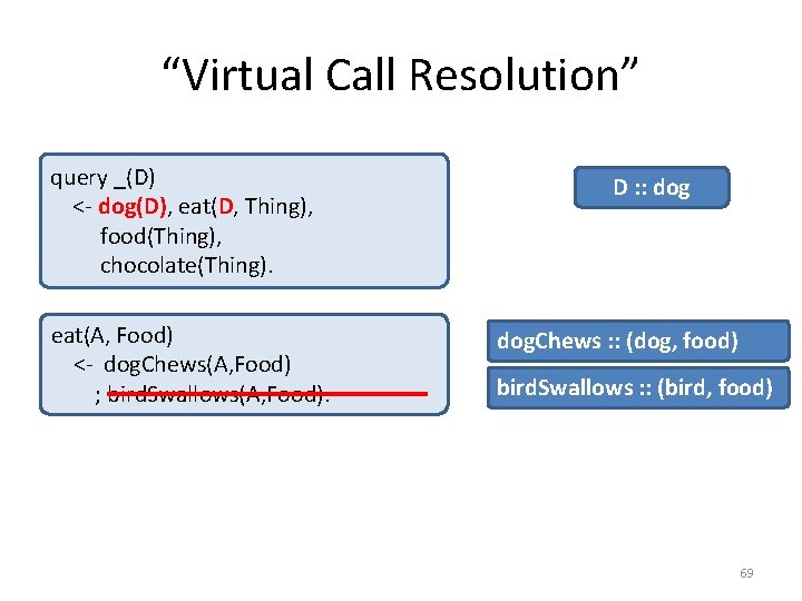
“Virtual Call Resolution” query _(D) <- dog(D), eat(D, Thing), food(Thing), chocolate(Thing). eat(A, Food) <- dog. Chews(A, Food) ; bird. Swallows(A, Food). D : : dog. Chews : : (dog, food) bird. Swallows : : (bird, food) 69

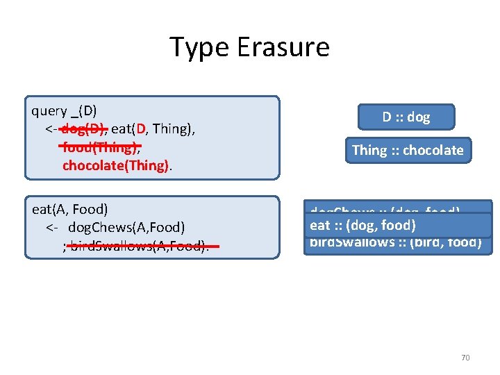
Type Erasure query _(D) <- dog(D), eat(D, Thing), food(Thing), chocolate(Thing). eat(A, Food) <- dog. Chews(A, Food) ; bird. Swallows(A, Food). D : : dog Thing : : chocolate dog. Chews : : (dog, food) eat : : (dog, food) bird. Swallows : : (bird, food) 70

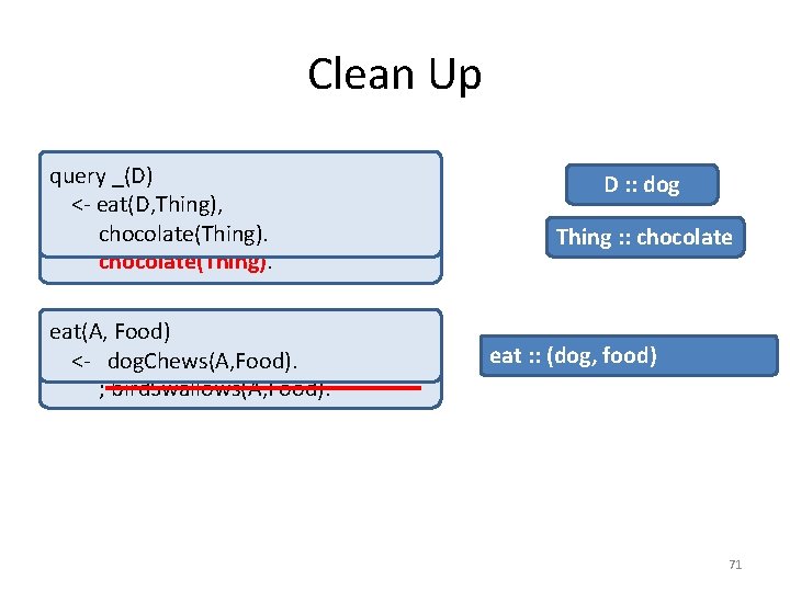
Clean Up query _(D) dog(D), eat(D, Thing), <- eat(D, Thing), food(Thing), chocolate(Thing). eat(A, Food) dog. Chews(A, Food) <- dog. Chews(A, Food). ; bird. Swallows(A, Food). D : : dog Thing : : chocolate eat : : (dog, food) 71

References on Datalog and Types • “Type inference for datalog and its application to query optimisation”, de Moor et al. , PODS ‘ 08 • “Type inference for datalog with complex type hierarchies”, Schafer and de Moor, POPL ‘ 10 • “Semantic Query Optimization in the Presence of Types”, Meier et al. , PODS ‘ 10 72

Datalog Program Analysis Systems • BDDBDDB – Data structure: BDD • Semmle (. QL) – Object-oriented syntax – No update • Doop – Points-to analysis for full Java – Supports for many variants of context and heap sensitivity. 73

REVIEW 74

Program Analysis • What is it? – Fundamental analysis aiding software development – Help make programs run fast, help you find bugs • Why in Datalog? – Declarative recursion • How does it work? – Really well! order of magnitude faster than handtuned, Java tools – Datalog optimizations are crucial in achieving performance 75

Program Analysis logic imperative functional Datalog understanding program behavior ^ • “Evita Raced: Meta-compilation for declarative networks”, Condie et al. , VLDB ‘ 08 76

OPEN CHALLENGES 77

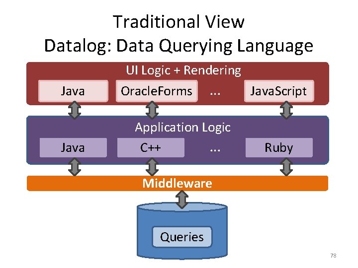
Traditional View Datalog: Data Querying Language UI Logic + Rendering Java Oracle. Forms … Application Logic … C++ Java. Script Ruby Middleware Queries 78

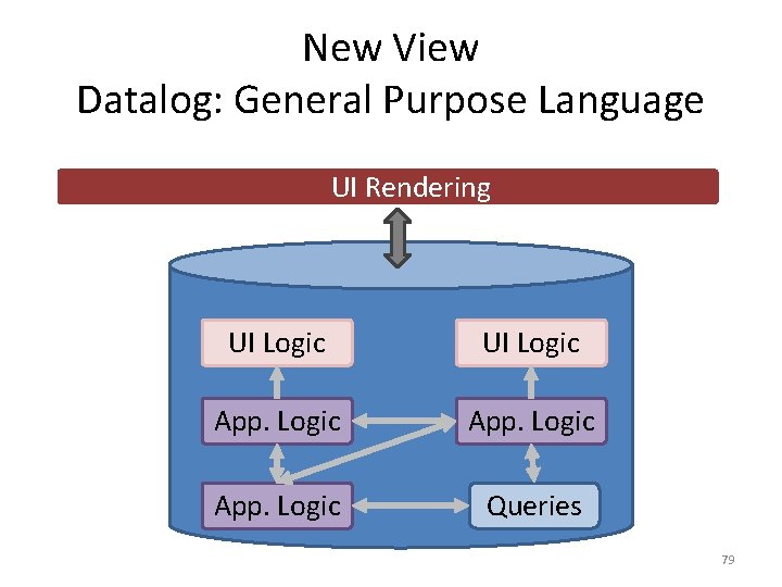
New View Datalog: General Purpose Language UI Rendering UI Logic App. Logic Queries 79

Challenges Raised by Program Analysis • Datalog Programming in the large – Modularization support – Reuse (generic programming) – Debugging and Testing • Expressiveness: – Recursion through negation, aggregation – Declarative state • Optimization, optimization – In the presence of recursion! 80

Acknowledgements • Slides: – Martin Bravenboer & Logic. Blox, Inc. – Damien Sereni & Semmle, Inc. – Matt Might, University of Utah 81

Outline of Tutorial June 14, 2011: The Second Coming of Datalog! • • • Refresher: basics of Datalog Application #1: Data Integration and Exchange Application #2: Program Analysis Application #3: Declarative Networking Conclusions 82

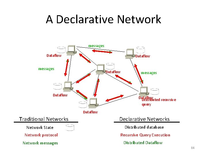
Declarative Networking • A declarative framework for networks: – Declarative language: “ask for what you want, not how to implement it” – Declarative specifications of networks, compiled to distributed dataflows – Runtime engine to execute distributed dataflows • Observation: Recursive queries are a natural fit for routing 83

A Declarative Network messages Dataflow messages Dataflow Distributed recursive query Dataflow Traditional Networks Declarative Networks Network State Distributed database Network protocol Recursive Query Execution Network messages Distributed Dataflow 84

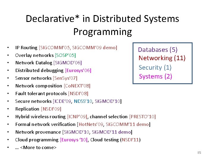
Declarative* in Distributed Systems Programming • • • • IP Routing [SIGCOMM’ 05, SIGCOMM’ 09 demo] Databases (5) Overlay networks [SOSP’ 05] Networking (11) Network Datalog [SIGMOD’ 06] Security (1) Distributed debugging [Eurosys’ 06] Systems (2) Sensor networks [Sen. Sys’ 07] Network composition [Co. NEXT’ 08] Fault tolerant protocols [NSDI’ 08] Secure networks [ICDE’ 09, NDSS’ 10, SIGMOD’ 10] Replication [NSDI’ 09] Hybrid wireless routing [ICNP’ 09], channel selection [PRESTO’ 10] Formal network verification [Hot. Nets’ 09, SIGCOMM’ 11 demo] Network provenance [SIGMOD’ 10, SIGMOD’ 11 demo] Cloud programming [Eurosys ‘ 10], Cloud testing (NSDI’ 11) … <More to come> 85

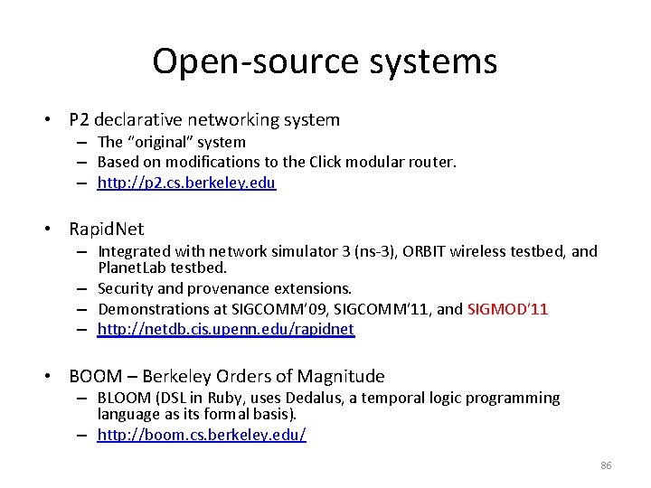
Open-source systems • P 2 declarative networking system – The “original” system – Based on modifications to the Click modular router. – http: //p 2. cs. berkeley. edu • Rapid. Net – Integrated with network simulator 3 (ns-3), ORBIT wireless testbed, and Planet. Lab testbed. – Security and provenance extensions. – Demonstrations at SIGCOMM’ 09, SIGCOMM’ 11, and SIGMOD’ 11 – http: //netdb. cis. upenn. edu/rapidnet • BOOM – Berkeley Orders of Magnitude – BLOOM (DSL in Ruby, uses Dedalus, a temporal logic programming language as its formal basis). – http: //boom. cs. berkeley. edu/ 86

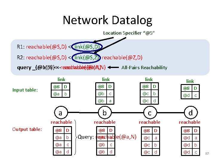
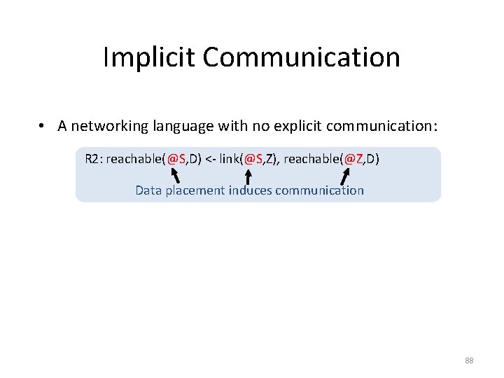
Network Datalog Location Specifier “@S” R 1: reachable(@S, D) <- link(@S, D) R 2: reachable(@S, D) <- link(@S, Z), reachable(@Z, D) query _(@M, N) reachable(@M, N) _(@a, N) <-<-reachable(@a, N) link Input table: Output table: All-Pairs Reachability link @S D @a b @b c @c b @d c @b a @c d a b c d reachable @S D @a b @a c @b @a d @b @S D @c a @d a c @c b @d b d @c d @d c Query: reachable(@a, N) @b a 87

Implicit Communication • A networking language with no explicit communication: R 2: reachable(@S, D) <- link(@S, Z), reachable(@Z, D) Data placement induces communication 88

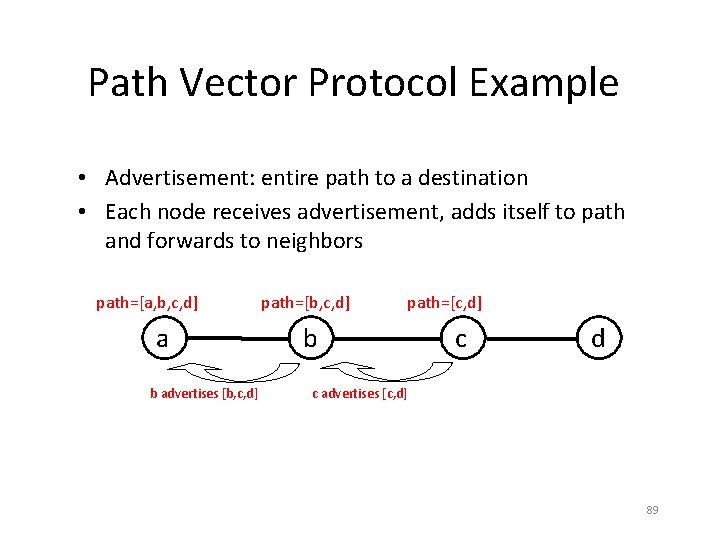
Path Vector Protocol Example • Advertisement: entire path to a destination • Each node receives advertisement, adds itself to path and forwards to neighbors path=[a, b, c, d] a b advertises [b, c, d] path=[c, d] b c d c advertises [c, d] 89

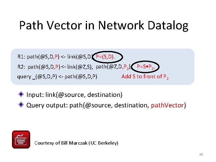
Path Vector in Network Datalog R 1: path(@S, D, P) <- link(@S, D), P=(S, D). R 2: path(@S, D, P) <- link(@Z, S), path(@Z, D, P 2), P=S P 2. query _(@S, D, P) <- path(@S, D, P) Add S to front of P 2 Input: link(@source, destination) Query output: path(@source, destination, path. Vector) Courtesy of Bill Marczak (UC Berkeley) 90

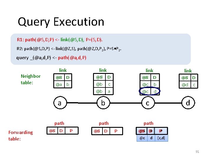
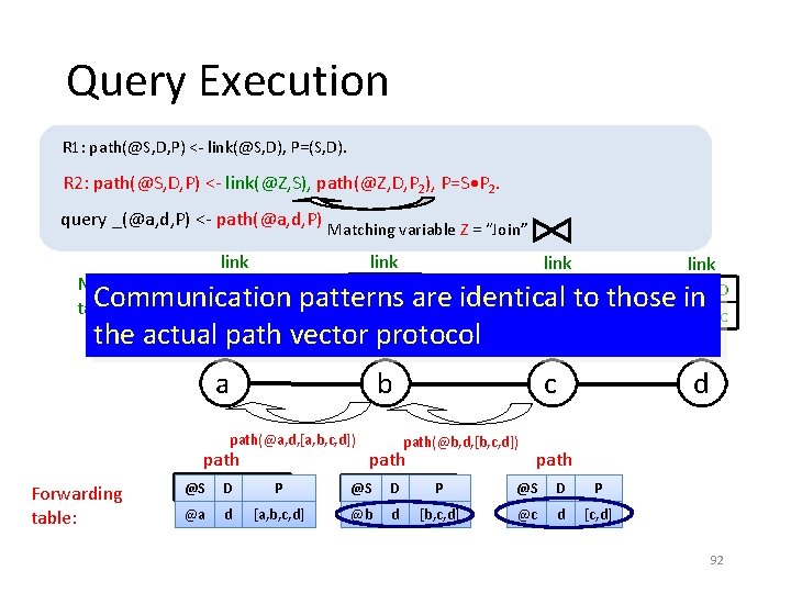
Query Execution R 1: path(@S, D, P) <- link(@S, D), P=(S, D). R 2: path(@S, D, P) <- link(@Z, S), path(@Z, D, P 2), P=S P 2. query _(@a, d, P) <- path(@a, d, P) link Neighbor table: Forwarding table: link @S D @a b @b c @c b @d c @b a @c d a b c path @S link D P @S D P d @S D D @S @c d PP [c, d] 91

Query Execution R 1: path(@S, D, P) <- link(@S, D), P=(S, D). R 2: path(@S, D, P) <- link(@Z, S), path(@Z, D, P 2), P=S P 2. query _(@a, d, P) <- path(@a, d, P) Matching variable Z = “Join” link Neighbor @S D Communication table: @a b link @S D @S patterns are identical to those in @b c @c b @d the actual path vector@bprotocol a @c d a b path(@a, d, [a, b, c, d]) path Forwarding table: @S D @a d PP [a, b, c, d] c path(@b, d, [b, c, d]) path D c d path @S D PP @S D P @b d [b, c, d] @c d [c, d] 92

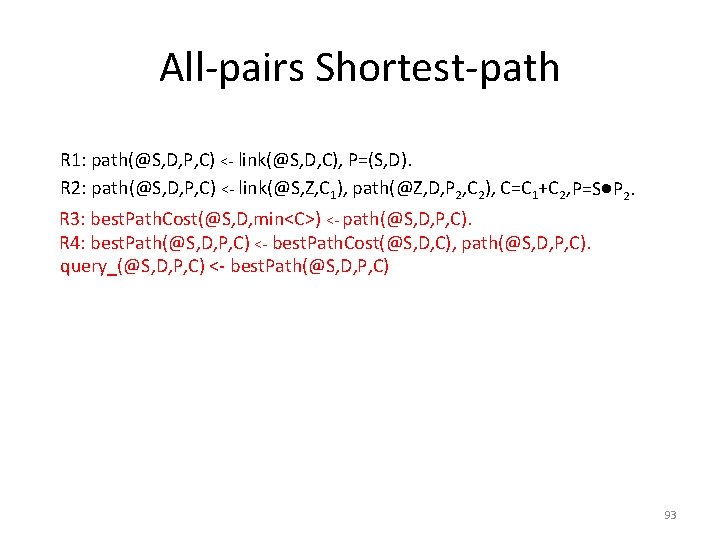
All-pairs Shortest-path R 1: path(@S, D, P, C) <- link(@S, D, C), P=(S, D). R 2: path(@S, D, P, C) <- link(@S, Z, C 1), path(@Z, D, P 2, C 2), C=C 1+C 2, P=S P 2. R 3: best. Path. Cost(@S, D, min<C>) <- path(@S, D, P, C). R 4: best. Path(@S, D, P, C) <- best. Path. Cost(@S, D, C), path(@S, D, P, C). query_(@S, D, P, C) <- best. Path(@S, D, P, C) 93

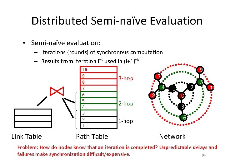
Distributed Semi-naïve Evaluation • Semi-naïve evaluation: – Iterations (rounds) of synchronous computation – Results from iteration ith used in (i+1)th 10 9 8 7 6 5 4 3 2 1 Link Table Path Table 9 7 3 -hop 4 8 2 -hop 1 2 5 10 0 3 6 Network Problem: How do nodes know that an iteration is completed? Unpredictable delays and failures make synchronization difficult/expensive. 94

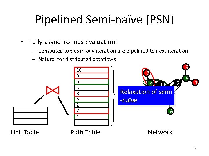
Pipelined Semi-naïve (PSN) • Fully-asynchronous evaluation: – Computed tuples in any iteration are pipelined to next iteration – Natural for distributed dataflows 9 10 7 9 5 6 2 4 1 3 8 of semi 0 Relaxation 8 5 2 7 4 1 Link Table Path Table -naïve 10 3 6 Network 95

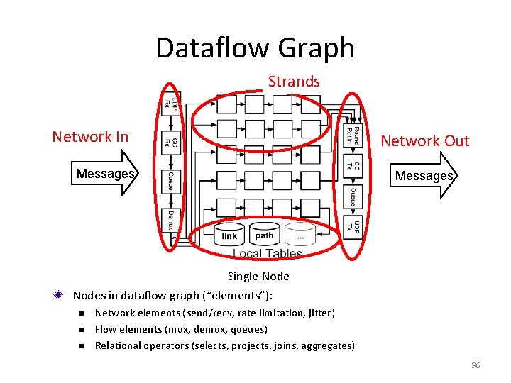
Dataflow Graph Strands Network In Network Out Messages Single Nodes in dataflow graph (“elements”): n n n Network elements (send/recv, rate limitation, jitter) Flow elements (mux, demux, queues) Relational operators (selects, projects, joins, aggregates) 96

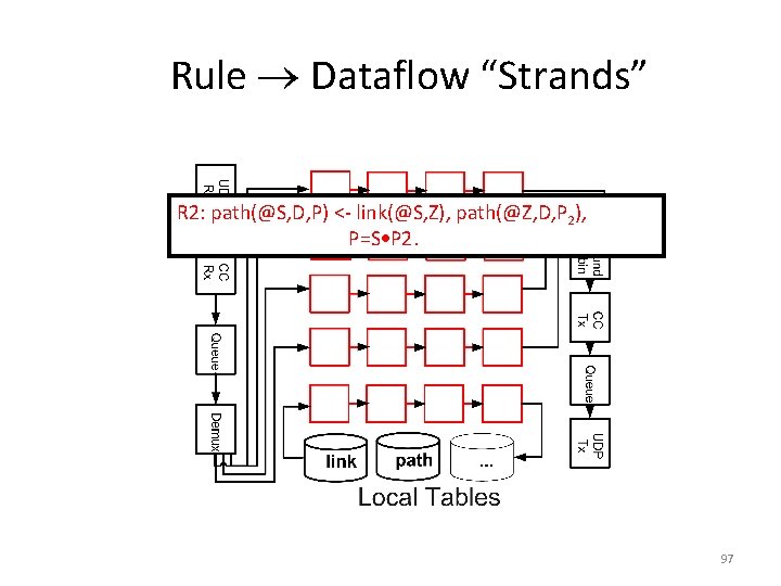
Rule Dataflow “Strands” R 2: path(@S, D, P) <- link(@S, Z), path(@Z, D, P 2), P=S P 2. 97

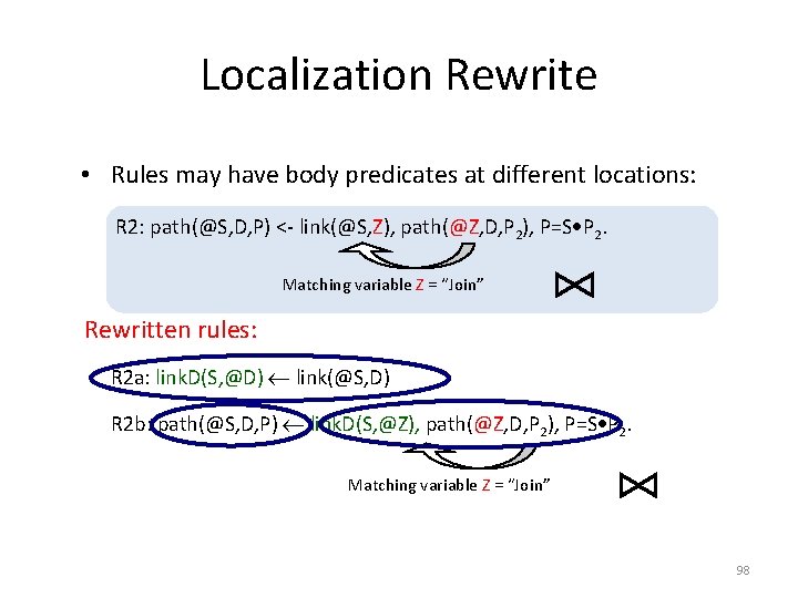
Localization Rewrite • Rules may have body predicates at different locations: R 2: path(@S, D, P) <- link(@S, Z), path(@Z, D, P 2), P=S P 2. Matching variable Z = “Join” Rewritten rules: R 2 a: link. D(S, @D) link(@S, D) R 2 b: path(@S, D, P) link. D(S, @Z), path(@Z, D, P 2), P=S P 2. Matching variable Z = “Join” 98

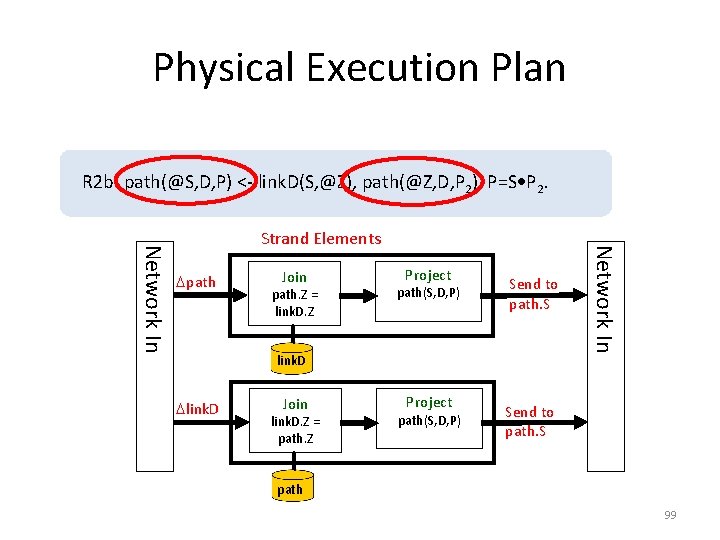
Physical Execution Plan R 2 b: path(@S, D, P) <- link. D(S, @Z), path(@Z, D, P 2), P=S P 2. path Join path. Z = link. D. Z Project path(S, D, P) Send to path. S link. D Join link. D. Z = path. Z Project path(S, D, P) Network In Strand Elements Send to path. S path 99

Pipelined Evaluation • Challenges: – Does PSN produce the correct answer? – Is PSN bandwidth efficient? • I. e. does it make the minimum number of inferences? • Theorems [SIGMOD’ 06]: – RSSN(p) = RSPSN(p), where RS is results set – No repeated inferences in computing RSPSN(p) – Require per-tuple timestamps in delta rules and FIFO and reliable channels 100

Incremental View Maintenance • Leverages insertion and deletion delta rules for state modifications. • Complications arise from duplicate evaluations. • Consider the Reachable query. What if there are many ways to route between two nodes a and b, i. e. many possible derivations for reachable(a, b)? • Mechanisms: still use delta rules, but additionally, apply – Count algorithm (for non-recursive queries). – Delete and Rederive (SIGMOD’ 93). Expensive in distributed settings. Maintaining Views Incrementally. Gupta, Mumick, Ramakrishnan, Subrahmanian. SIGMOD 1993. 101

Recent PSN Enhancements • Provenance-based approach – Condensed form of provenance piggy-backed with each tuple for derivability test. – Recursive Computation of Regions and Connectivity in Networks. Liu, Taylor, Zhou, Ives, and Loo. ICDE 2009. • Relaxation of FIFO requirements: – Maintaining Distributed Logic Programs Incrementally. Vivek Nigam, Limin Jia, Boon Thau Loo and Andre Scedrov. 13 th International ACM SIGPLAN Symposium on Principles and Practice of Declarative Programming (PPDP), 2011. 102

Optimizations • Traditional: – Aggregate Selections – Magic Sets rewrite – Predicate Reordering PV/DV DSR • New: – Multi-query optimizations: • Query Results caching • Opportunistic message sharing – Cost-based optimizations • Network statistics (e. g. density, route request rates, etc. ) • Combining top-down and bottom-up evaluation 103

Suggested Readings • Networking use cases: – Declarative Routing: Extensible Routing with Declarative Queries. Loo, Hellerstein, Stoica, and Ramakrishnan. SIGCOMM 2005. – Implementing Declarative Overlays. Loo, Condie, Hellerstein, Maniatis, Roscoe, and Stoica. SOSP 2005. • Distributed recursive query processing: – *Declarative Networking: Language, Execution and Optimization. Loo, Condie, Garofalakis, Gay, Hellerstein, Maniatis, Ramakrishnan, Roscoe, and Stoica, SIGMOD 06. – Recursive Computation of Regions and Connectivity in Networks. Liu, Taylor, Zhou, Ives, and Loo. ICDE 2009. 104

Challenges and Opportunities • Declarative networking adoption: – Leverage well-known open-source software-based projects, e. g. ns-3, Quagga, Open. Flow – Wrappers for legacy code – Usability studies – Open-source code release and demonstrations • Formal network verification: – Integration of formal tools (e. g. theorem provers, SMT solvers), formal network models (e. g. routing algebra) – Operational semantics of Network Datalog and subsequent extensions – Other properties: timing, security • Opportunities for automated program synthesis 105

Outline of Tutorial June 14, 2011: The Second Coming of Datalog! • • • Refresher: basics of Datalog Application #1: Data Integration and Exchange Application #2: Program Analysis Application #3: Declarative Networking Modern System Implementations Open Questions 106

Outline of Tutorial June 14, 2011: The Second Coming of Datalog! • • • Refresher: basics of Datalog Application #1: Data Integration and Exchange Application #2: Program Analysis Application #3: Declarative Networking Conclusions 111

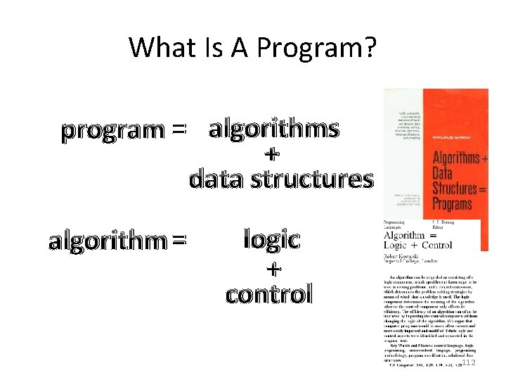
What Is A Program? program = algorithms + data structures algorithm = logic + control 112

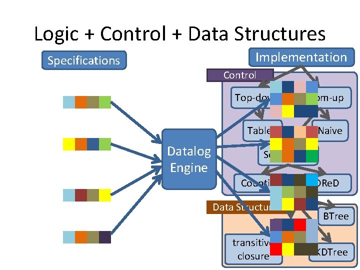
Logic + Control + Data Structures Implementation Specifications Control Datalog Engine Top-down Bottom-up Tabled Naive Semi-naive Counting Data Structures BDDs transitive closure DRe. D BTree KDTree 113

THE END… OR IS IT THE BEGINNING? 114

Backup 115

Aggregate Selections • Prune communication using running state of monotonic aggregate – Avoid sending tuples that do not affect value of agg – E. g. , shortest-paths query • Challenge in distributed setting: – Out-of-order (in terms of monotonic aggregate) arrival of tuples – Solution: Periodic aggregate selections • Buffer up tuples, periodically send best-agg tuples 117

Academic • Coral (1990 – 1997) – Semantics: insert/delete/update, modules, multisets – Evaluation: magic sets, indexing, materialization • LDL++ (? – 1999) – Semantics: complex terms, multisets, user-defined aggregates, updates – Evaluation: top-down evaluation • Rapid. Net declarative networking (2007 - present) – Semantics: Datalog with distribution – Evaluation: Pipelined semi-naïve evaluation • Bloom (2009 – present) – Semantics: Datalog with time: next, prev, async 118

Other Relevant References • Magic sets – “Cost-based Optimization for Magic: Algebra and Implementation”, Seshadri et al. , SIGMOD ’ 96 – “Adding Magic to an Optimising Datalog Compiler”, Sereni, Avgustinov, and de Moor, SIGMOD ’ 08 • Program analysis with Datalog – “Strictly Declarative Specification of Sophisticated Pointsto Analyses”, Bravenboer et al. , OOPSLA ’ 08 – “Context Sensitive Program Analysis as Database Queries”, Lam et al. , PODS ‘ 05 119

Many Ways To Analyze Programs • • points-to abstract interpretation type-based pattern-based 120

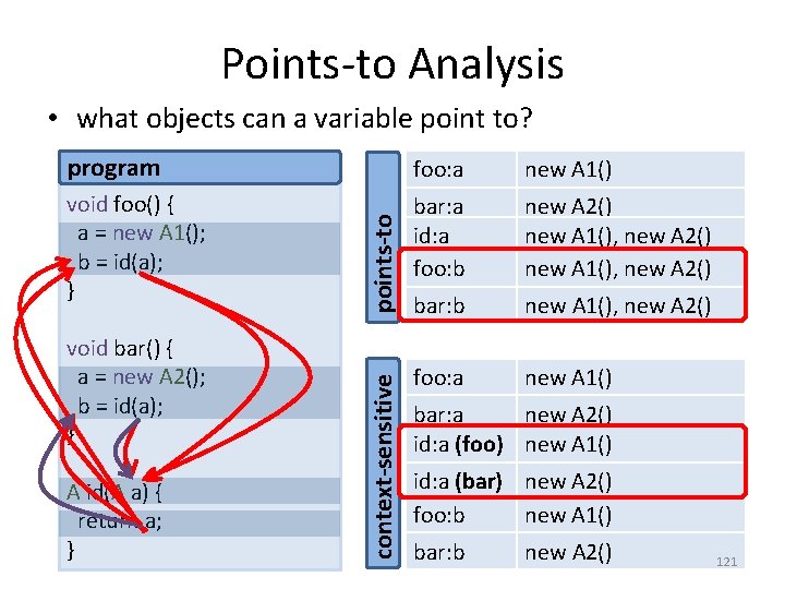
Points-to Analysis • what objects can a variable point to? foo: a new A 1() void foo() { a = new A 1(); b = id(a); } bar: a id: a foo: b new A 2() new A 1(), new A 2() bar: b new A 1(), new A 2() foo: a new A 1() A id(A a) { return a; } context-sensitive void bar() { a = new A 2(); b = id(a); } points-to program bar: a new A 2() id: a (foo) new A 1() id: a (bar) new A 2() foo: b new A 1() bar: b new A 2() 121

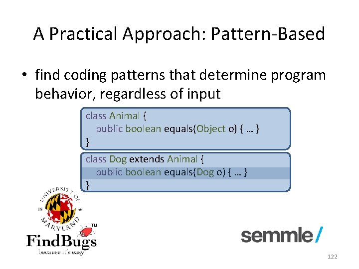
A Practical Approach: Pattern-Based • find coding patterns that determine program behavior, regardless of input class Animal { public boolean equals(Object o) { … } } class Dog extends Animal { public boolean equals(Dog o) { … } } 122

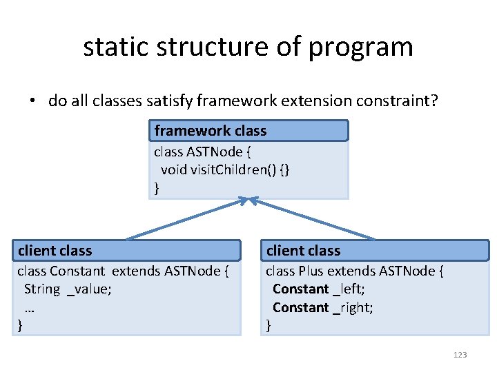
static structure of program • do all classes satisfy framework extension constraint? framework class ASTNode { void visit. Children() {} } client class Constant extends ASTNode { String _value; … } class Plus extends ASTNode { Constant _left; Constant _right; } 123

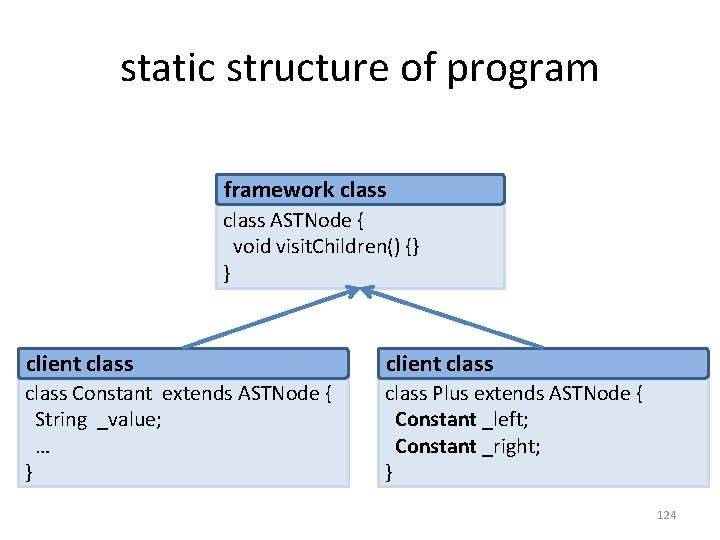
static structure of program framework class ASTNode { void visit. Children() {} } client class Constant extends ASTNode { String _value; … } class Plus extends ASTNode { Constant _left; Constant _right; } 124

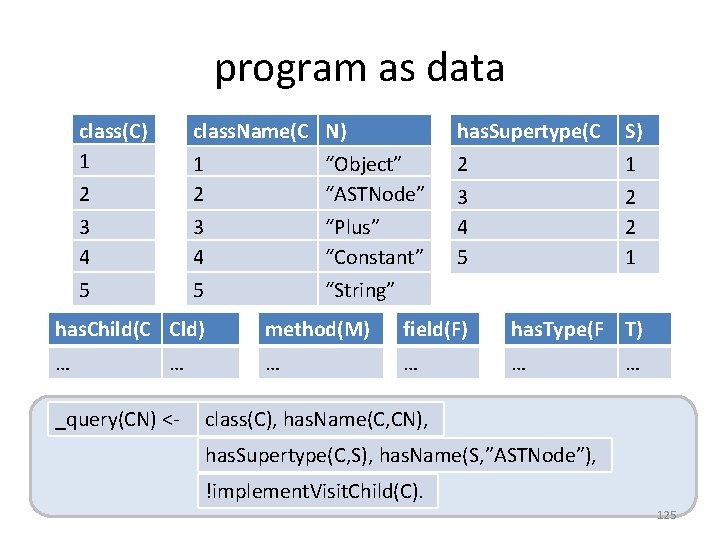
program as data class(C) 1 2 class. Name(C N) 1 “Object” 2 “ASTNode” 3 4 5 “Plus” “Constant” “String” has. Supertype(C 2 S) 1 3 4 5 2 2 1 has. Child(C Cld) method(M) field(F) has. Type(F T) … … … _query(CN) <- … class(C), has. Name(C, CN), has. Supertype(C, S), has. Name(S, ”ASTNode”), !implement. Visit. Child(C). 125

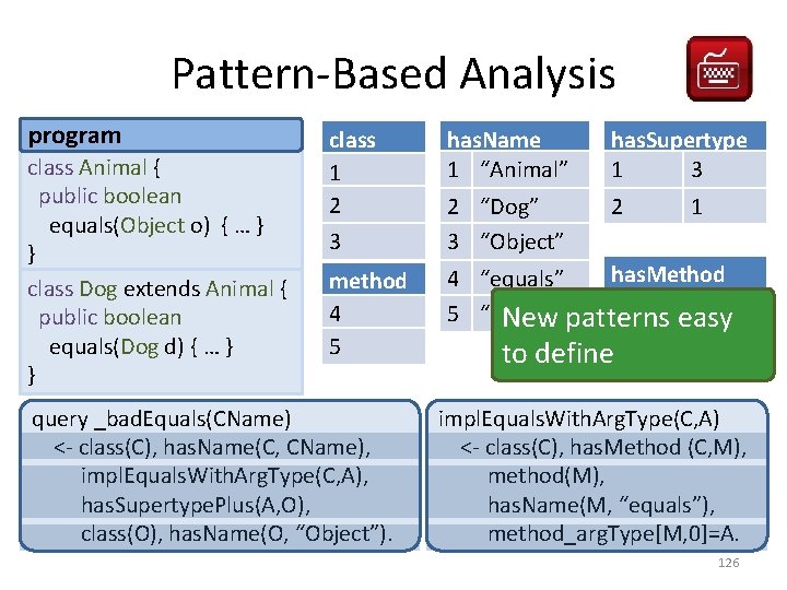
Pattern-Based Analysis program class Animal { public boolean equals(Object o) { … } } class Dog extends Animal { public boolean equals(Dog d) { … } } class 1 2 has. Name 1 “Animal” has. Supertype 1 3 2 “Dog” 3 “Object” method 4 5 has. Method 4 “equals” 1 4 5 “equals” New patterns easy 5 to define 2 query _bad. Equals(CName) <- class(C), has. Name(C, CName), impl. Equals. With. Arg. Type(C, A), has. Supertype. Plus(A, O), class(O), has. Name(O, “Object”). 1 impl. Equals. With. Arg. Type(C, A) <- class(C), has. Method (C, M), method(M), has. Name(M, “equals”), method_arg. Type[M, 0]=A. 126

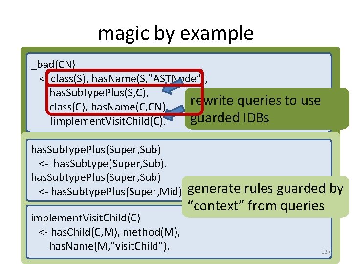
magic by example _bad(CN) <- class(S), has. Name(S, ”ASTNode”), has. Subtype. Plus(S, C), rewrite queries to use class(C), has. Name(C, CN), guarded IDBs !implement. Visit. Child(C). has. Subtype. Plus(Super, Sub) <- has. Subtype(Super, Sub). has. Subtype. Plus(Super, Sub) rules guarded by <- has. Subtype. Plus(Super, Mid), generate has. Supertype(Mid, Sub). implement. Visit. Child(C) <- has. Child(C, M), method(M), has. Name(M, ”visit. Child”). “context” from queries 127

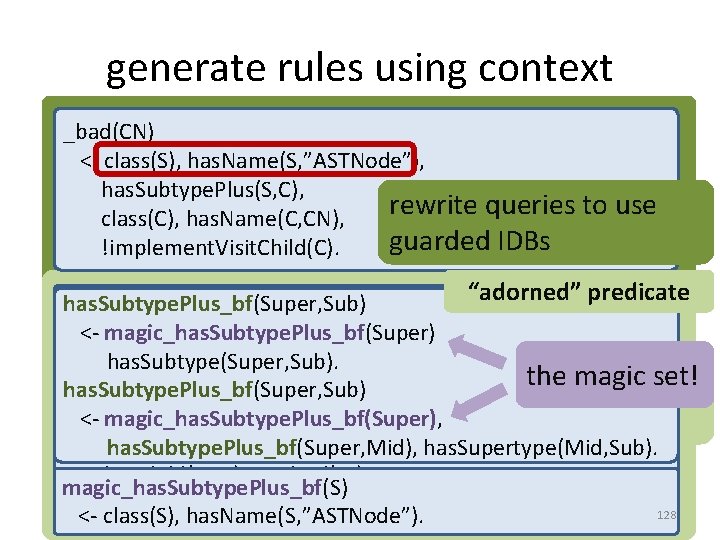
generate rules using context _bad(CN) <- class(S), has. Name(S, ”ASTNode”), has. Subtype. Plus(S, C), rewrite queries to use class(C), has. Name(C, CN), guarded IDBs !implement. Visit. Child(C). “adorned” predicate has. Subtype. Plus_bf(Super, Sub) <- class(S), magic_has. Subtype. Plus_bf(Super) has. Name(S, ”ASTNode”), has. Subtype(Super, Sub). <has. Subtype. Plus(Super, Sub) has. Subtype(Super, Sub). has. Subtype. Plus_bf(Super, Sub) theguarded magic set! generate rules <- has. Subtype. Plus(Super, Mid), has. Supertype(Mid, Sub). has. Subtype. Plus_bf(Super, Sub) has. Subtype. Plus_bf(Super, Mid), has. Supertype(Mid, Sub). by <- has. Subtype. Plus_bf(Super, Mid), class(S), magic_has. Subtype. Plus_bf(Super), has. Name(S, ”ASTNode”), has. Supertype(Mid, Sub). “context” from queries implement. Visit. Child(C) has. Subtype. Plus_bf(Super, Mid), has. Supertype(Mid, Sub). <- has. Child(C, M), method(M), magic_has. Subtype. Plus_bf(S) has. Name(M, ”visit. Child”). 128 <- class(S), has. Name(S, ”ASTNode”).

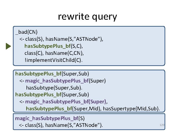
rewrite query _bad(CN) <- class(S), has. Name(S, ”ASTNode”), has. Subtype. Plus(S, C), has. Subtype. Plus_bf(S, C), class(C), has. Name(C, CN), !implement. Visit. Child(C). has. Subtype. Plus_bf(Super, Sub) <- magic_has. Subtype. Plus_bf(Super) has. Subtype(Super, Sub). has. Subtype. Plus_bf(Super, Sub) <- magic_has. Subtype. Plus_bf(Super), has. Subtype. Plus_bf(Super, Mid), has. Supertype(Mid, Sub). magic_has. Subtype. Plus_bf(S) <- class(S), has. Name(S, ”ASTNode”). 129

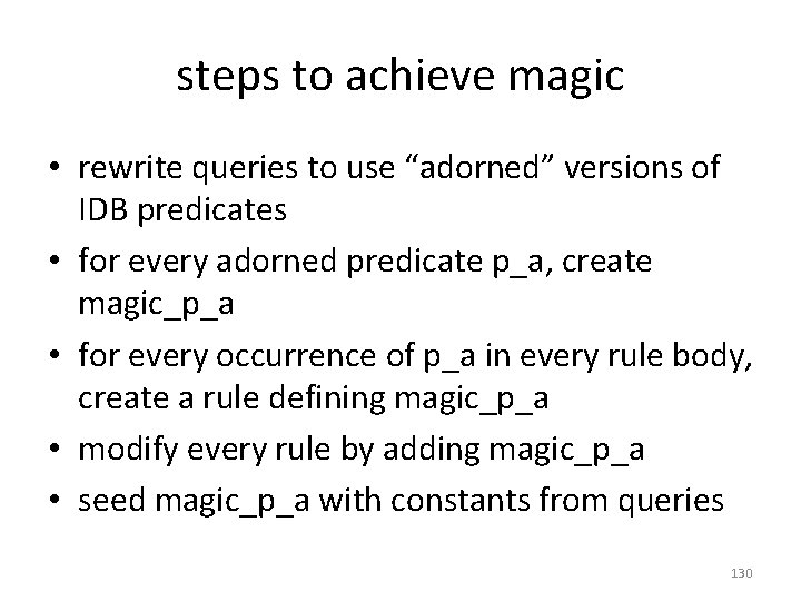
steps to achieve magic • rewrite queries to use “adorned” versions of IDB predicates • for every adorned predicate p_a, create magic_p_a • for every occurrence of p_a in every rule body, create a rule defining magic_p_a • modify every rule by adding magic_p_a • seed magic_p_a with constants from queries 130

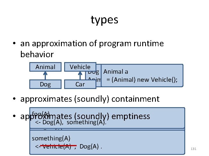
types • an approximation of program runtime behavior Animal Dog Vehicle Dog a. Dog Animal = new a Dog(); Animal a = new Vehicle(); Animal=animal (Animal) = a. Dog; new Vehicle(); Car • approximates (soundly) containment foo(A) • approximates (soundly) emptiness <- Dog(A), something(A). Animal(A), Dog(A), something(A). <- Vehicle(A) ; Dog(A). 131

MAGIC SETS 132

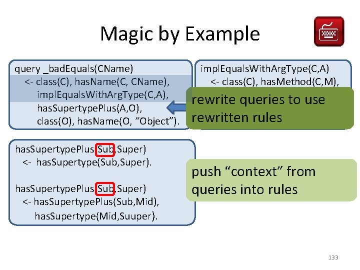
Magic by Example query _bad. Equals(CName) <- class(C), has. Name(C, CName), impl. Equals. With. Arg. Type(C, A), has. Supertype. Plus(A, O), class(O), has. Name(O, “Object”). has. Supertype. Plus(Sub, Super) <- has. Supertype(Sub, Super). has. Supertype. Plus(Sub, Super) <- has. Supertype. Plus(Sub, Mid), has. Supertype(Mid, Suuper). impl. Equals. With. Arg. Type(C, A) <- class(C), has. Method(C, M), method(M), rewrite queries to use has. Name(M, “equals”), rewritten rules method_arg. Type[M, 0]=A. push “context” from queries into rules 133

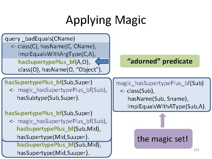
Applying Magic query _bad. Equals(CName) <- class(C), has. Name(C, CName), impl. Equals. With. Arg. Type(C, A), has. Supertype. Plus(A, O), has. Supertype. Plus_bf(A, O), class(O), has. Name(O, “Object”). has. Supertype. Plus_bf(Sub, Super) <- class(Sub), magic_has. Supertype. Plus_bf(Sub), has. Name(Sub, Sname), <- has. Subtype(Sub, Super). impl. Equals. With. Arg. Type(Sub, A), has. Subtype(Sub, Super). has. Supertype. Plus(Sub, Super) has. Supertype. Plus_bf(Sub, Super) <- has. Supertype. Plus(Sub, Mid), has. Supertype. Plus_bf(Sub, Mid), <- magic_has. Supertype. Plus_bf(Sub), has. Supertype. Plus_bf(Sub, Super) has. Supertype(Mid, Suuper). <- class(Sub), has. Name(Sub, Sname), has. Supertype. Plus_bf(Sub, Mid), impl. Equals. With. Arg. Type(Sub, A), has. Supertype(Mid, Suuper ). has. Supertype. Plus_bf(Sub, Mid), has. Supertype(Mid, Suuper). “adorned” predicate magic_has. Supertype. Plus_bf(Sub) <- class(Sub), has. Name(Sub, Sname), impl. Equals. With. AType(Sub, A). the magic set! 134

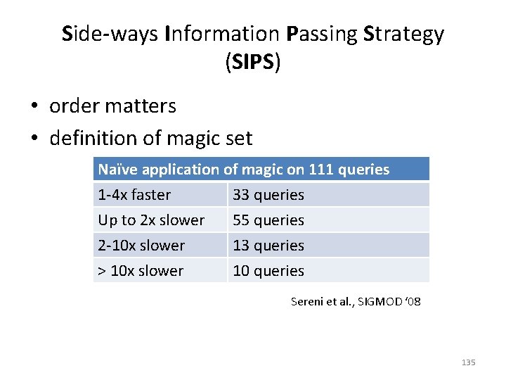
Side-ways Information Passing Strategy (SIPS) • order matters • definition of magic set _bad. Equals(CName) Naïvequery application of magic on 111 queries <- class(C), has. Supertype. Plus(A, O), has. Name(C, CName), 1 -4 x faster 33 queries impl. Equals. With. Arg. Type(C, A), class(C), has. Name(C, CName), Up to 2 x slower 55 queries impl. Equals. With. Arg. Type(C, A), has. Supertype. Plus(A, O), class(O), has. Name(O, 2 -10 x slower 13 queries“Object”). > 10 x slower 10 queries Sereni et al. , SIGMOD ‘ 08 135

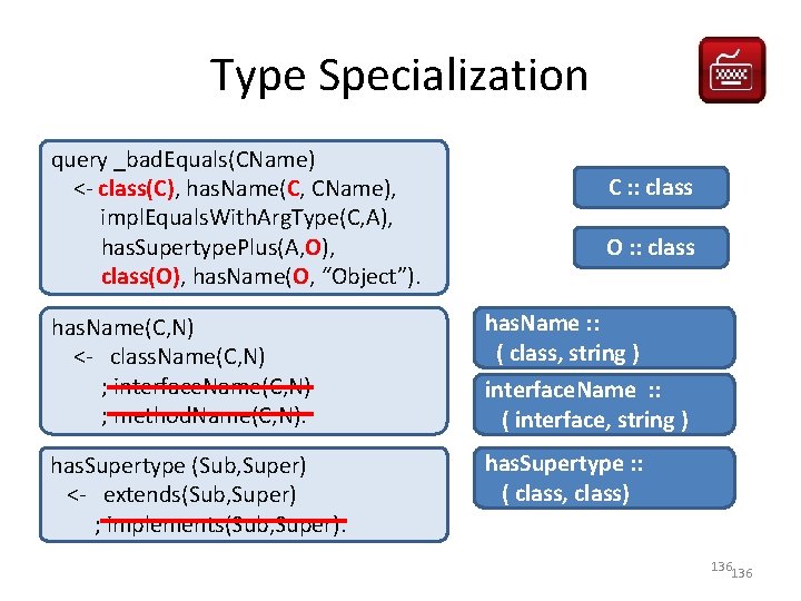
Type Specialization query _bad. Equals(CName) <- class(C), has. Name(C, CName), impl. Equals. With. Arg. Type(C, A), has. Supertype. Plus(A, O), class(O), has. Name(O, “Object”). C : : class O : : class has. Name(C, N) <- class. Name(C, N) ; interface. Name(C, N) ; method. Name(C, N). has. Name : : class. Name ( class, string ) has. Supertype (Sub, Super) <- extends(Sub, Super) ; implements(Sub, Super). has. Supertype : : ( class, class) interface. Name : : ( interface, string ) 136136

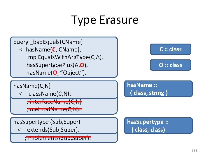
Type Erasure query _bad. Equals(CName) <- has. Name(C, class(C), has. Name(C, CName), impl. Equals. With. Arg. Type(C, A), has. Supertype. Plus(A, O), has. Name(O, class(O), has. Name(O, “Object”). C : : class O : : class has. Name(C, N) <- class. Name(C, N) ; interface. Name(C, N) ; method. Name(C, N). has. Name : : ( class, string ) has. Supertype (Sub, Super) extends(Sub, Super). <- extendeds(Sub, Super) ; implements(Sub, Super). has. Supertype : : ( class, class) 137

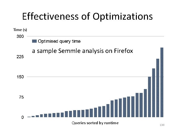
Effectiveness of Optimizations Time (s) a sample Semmle analysis on Firefox Queries sorted by runtime 138

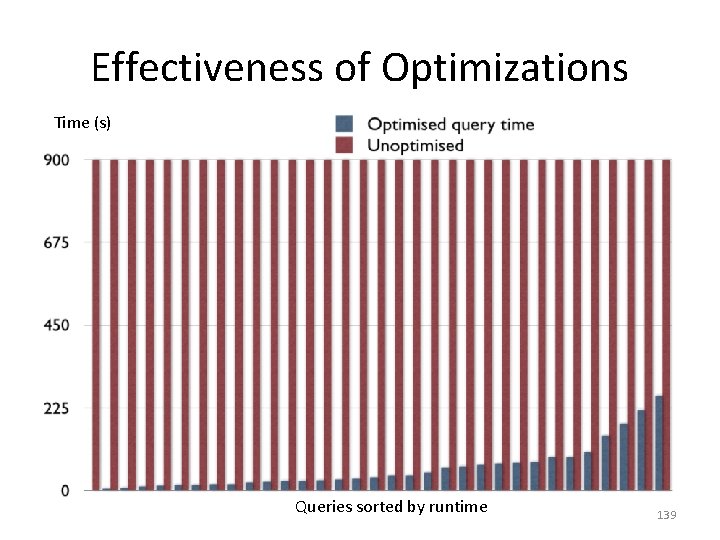
Effectiveness of Optimizations Time (s) Queries sorted by runtime 139

Type-enabled Optimizations it’s a Dog class Dog { void eat(Food f) { … } } it’s Chocolate animal. eat( (Food) thing); virtual call resolution type erasure 140