4 Datalog Queries Datalog query a finite set

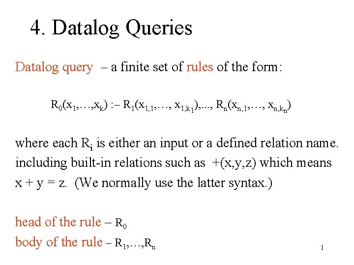
4. Datalog Queries Datalog query – a finite set of rules of the form: R 0(x 1, …, xk) : – R 1(x 1, 1, …, x 1, k 1), . . . , Rn(xn, 1, …, xn, kn) where each Ri is either an input or a defined relation name. including built-in relations such as +(x, y, z) which means x + y = z. (We normally use the latter syntax. ) head of the rule – R 0 body of the rule – R 1, …, Rn 1

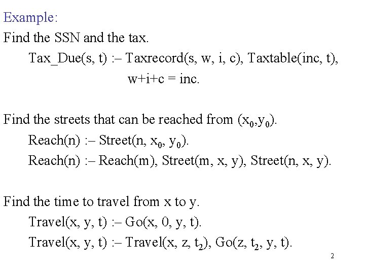
Example: Find the SSN and the tax. Tax_Due(s, t) : – Taxrecord(s, w, i, c), Taxtable(inc, t), w+i+c = inc. Find the streets that can be reached from (x 0, y 0). Reach(n) : – Street(n, x 0, y 0). Reach(n) : – Reach(m), Street(m, x, y), Street(n, x, y). Find the time to travel from x to y. Travel(x, y, t) : – Go(x, 0, y, t). Travel(x, y, t) : – Travel(x, z, t 2), Go(z, t 2, y, t). 2

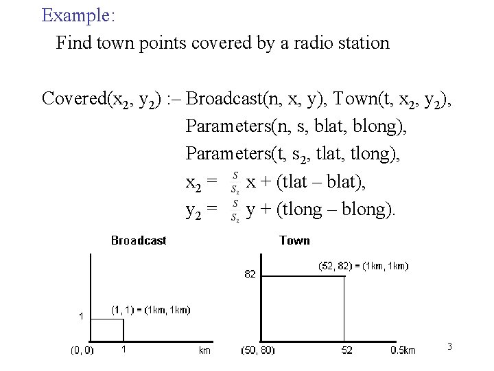
Example: Find town points covered by a radio station Covered(x 2, y 2) : – Broadcast(n, x, y), Town(t, x 2, y 2), Parameters(n, s, blat, blong), Parameters(t, s 2, tlat, tlong), x 2 = x + (tlat – blat), y 2 = y + (tlong – blong). 3

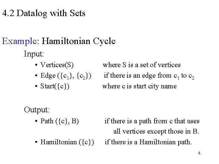
4. 2 Datalog with Sets Example: Hamiltonian Cycle Input: • Vertices(S) • Edge ({c 1}, {c 2}) • Start({c}) where S is a set of vertices if there is an edge from c 1 to c 2 where c is start city name Output: • Path ({c}, B) • Hamiltonian ({c}) if there is a path from c that uses all vertices except those in B. if there is a Hamiltonian path. 4

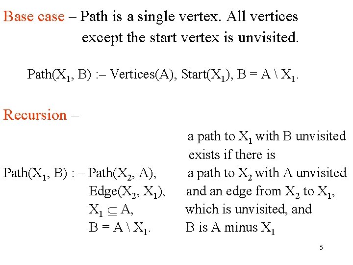
Base case – Path is a single vertex. All vertices except the start vertex is unvisited. Path(X 1, B) : – Vertices(A), Start(X 1), B = A X 1. Recursion – Path(X 1, B) : – Path(X 2, A), Edge(X 2, X 1), X 1 A, B = A X 1. a path to X 1 with B unvisited exists if there is a path to X 2 with A unvisited an edge from X 2 to X 1, which is unvisited, and B is A minus X 1 5

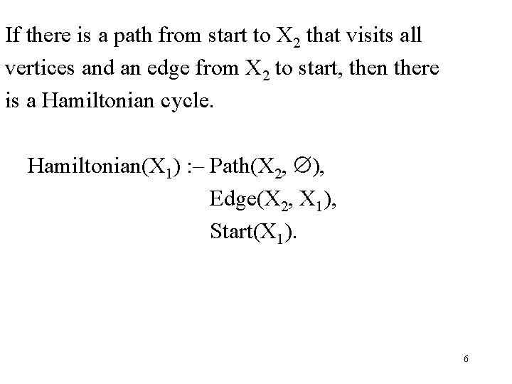
If there is a path from start to X 2 that visits all vertices and an edge from X 2 to start, then there is a Hamiltonian cycle. Hamiltonian(X 1) : – Path(X 2, ), Edge(X 2, X 1), Start(X 1). 6

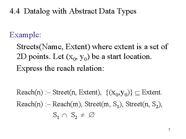
4. 4 Datalog with Abstract Data Types Example: Streets(Name, Extent) where extent is a set of 2 D points. Let (x 0, y 0) be a start location. Express the reach relation: Reach(n) : – Street(n, Extent), {(x 0, y 0)} Extent. Reach(n) : – Reach(m), Street(m, S 1), Street(n, S 2), S 1 S 2 7

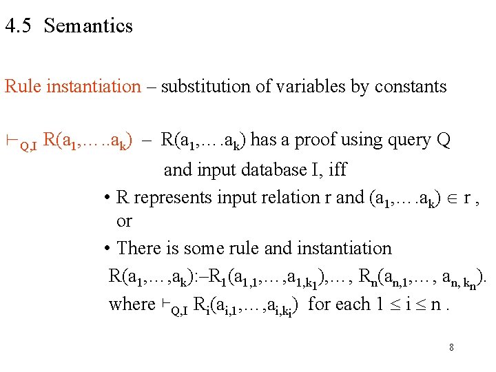
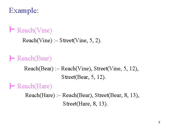
4. 5 Semantics Rule instantiation – substitution of variables by constants ⊢Q, I R(a 1, …. . ak) – R(a 1, …. ak) has a proof using query Q and input database I, iff • R represents input relation r and (a 1, …. ak) r , or • There is some rule and instantiation R(a 1, …, ak): –R 1(a 1, 1, …, a 1, k 1), …, Rn(an, 1, …, an, kn). where ⊢Q, I Ri(ai, 1, …, ai, ki) for each 1 i n. 8

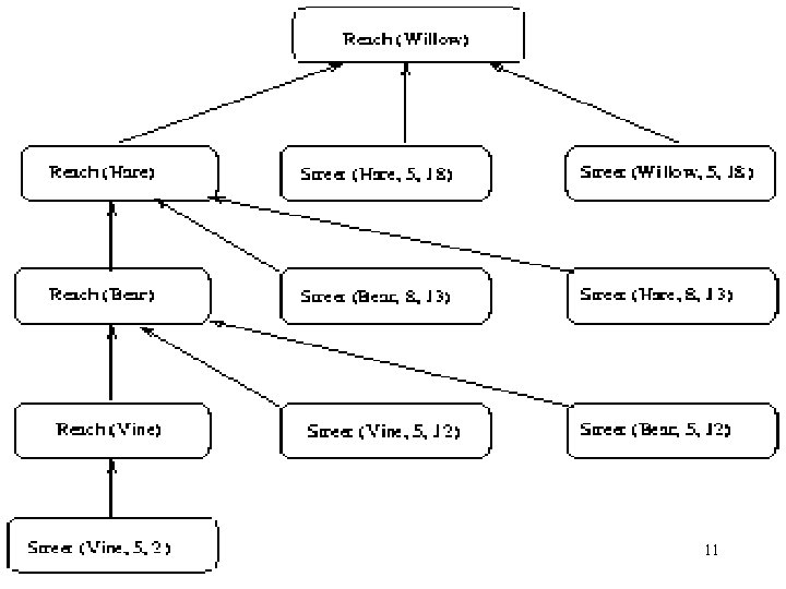
Example: Reach(Vine) : – Street(Vine, 5, 2). Reach(Bear) : – Reach(Vine), Street(Vine, 5, 12), Street(Bear, 5, 12). Reach(Hare) : – Reach(Bear), Street(Bear, 8, 13), Street(Hare, 8, 13). 9

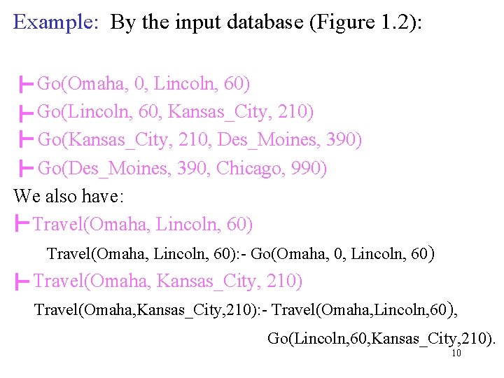
Example: By the input database (Figure 1. 2): Go(Omaha, 0, Lincoln, 60) Go(Lincoln, 60, Kansas_City, 210) Go(Kansas_City, 210, Des_Moines, 390) Go(Des_Moines, 390, Chicago, 990) We also have: Travel(Omaha, Lincoln, 60): - Go(Omaha, 0, Lincoln, 60) Travel(Omaha, Kansas_City, 210): - Travel(Omaha, Lincoln, 60), Go(Lincoln, 60, Kansas_City, 210). 10

11

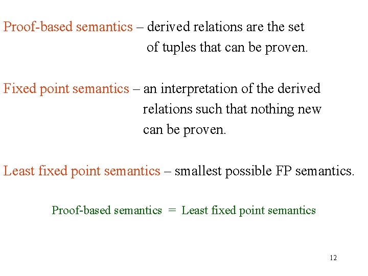
Proof-based semantics – derived relations are the set of tuples that can be proven. Fixed point semantics – an interpretation of the derived relations such that nothing new can be proven. Least fixed point semantics – smallest possible FP semantics. Proof-based semantics = Least fixed point semantics 12