Data Structures and Algorithm Analysis Algorithm Design Techniques

Data Structures and Algorithm Analysis Algorithm Design Techniques Lecturer: Jing Liu Email: neouma@mail. xidian. edu. cn Homepage: http: //see. xidian. edu. cn/faculty/liujing

The Greedy Approach n Greedy algorithms are usually designed to solve optimization problems in which a quantity is to be minimized or maximized. n n Greedy algorithms typically consist of a n iterative procedure that tries to find a local optimal solution. In some instances, these local optimal solutions translate to global optimal solutions. In others, they fail to give optimal solutions.

The Greedy Approach n n n A greedy algorithm makes a correct guess on the basis of little calculation without worrying about the future. Thus, it builds a solution step by step. Each step increases the size of the partial solution and is based on local optimization. The choice make is that which produces the largest immediate gain while maintaining feasibility. Since each step consists of little work based on a small amount of information, the resulting algorithms are typically efficient.

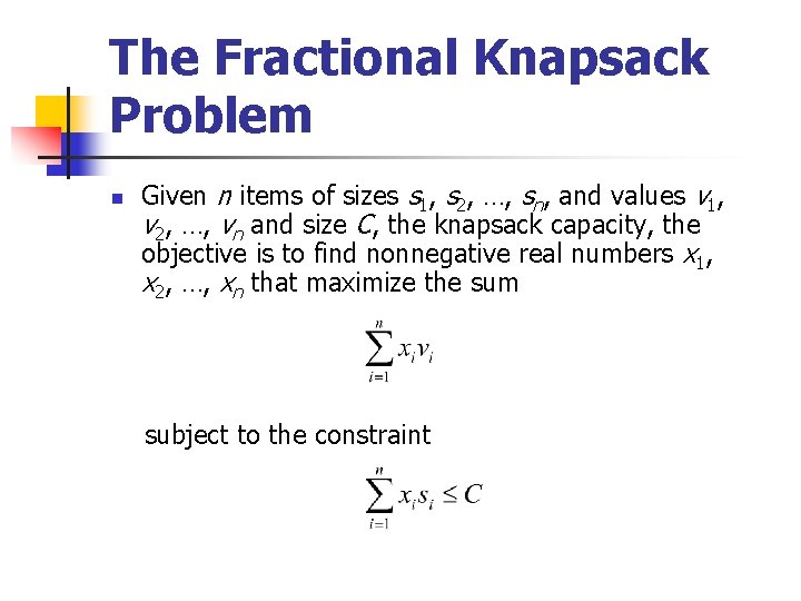
The Fractional Knapsack Problem n Given n items of sizes s 1, s 2, …, sn, and values v 1, v 2, …, vn and size C, the knapsack capacity, the objective is to find nonnegative real numbers x 1, x 2, …, xn that maximize the sum subject to the constraint

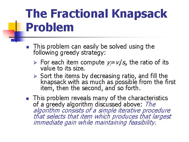
The Fractional Knapsack Problem n This problem can easily be solved using the following greedy strategy: For each item compute yi=vi/si, the ratio of its value to its size. Ø Sort the items by decreasing ratio, and fill the knapsack with as much as possible from the first item, then the second, and so forth. Ø n This problem reveals many of the characteristics of a greedy algorithm discussed above: The algorithm consists of a simple iterative procedure that selects that item which produces that largest immediate gain while maintaining feasibility.

File Compression n n Suppose we are given a file, which is a string of characters. We wish to compress the file as much as possible in such a way that the original file can easily be reconstructed. Let the set of characters in the file be C={c 1, c 2, …, cn}. Let also f(ci), 1 i n, be the frequency of character ci in the file, i. e. , the number of times ci appears in the file.

File Compression n n Using a fixed number of bits to represent each character, called the encoding of the character, the size of the file depends only on the number of characters in the file. Since the frequency of some characters may be much larger than others, it is reasonable to use variable length encodings.

File Compression n Intuitively, those characters with large frequencies should be assigned short encodings, whereas long encodings may be assigned to those characters with small frequencies. When the encodings vary in length, we stipulate that the encoding of one character must not be the prefix of the encoding of another character; such codes are called prefix codes. For instance, if we assign the encodings 10 and 101 to the letters “a” and “b”, there will be an ambiguity as to whether 10 is the encoding of “a” or is the prefix of the encoding of the letter “b”.

File Compression n n Once the prefix constraint is satisfied, the decoding becomes unambiguous; the sequence of bits is scanned until an encoding of some character is found. One way to “parse” a given sequence of bits is to use a full binary tree, in which each internal node has exactly two branches labeled by 0 an 1. The leaves in this tree corresponding to the characters. Each sequence of 0’s and 1’s on a path from the root to a leaf corresponds to a character encoding.

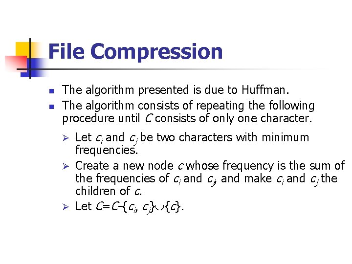
File Compression n n The algorithm presented is due to Huffman. The algorithm consists of repeating the following procedure until C consists of only one character. Let ci and cj be two characters with minimum frequencies. Ø Create a new node c whose frequency is the sum of the frequencies of ci and cj, and make ci and cj the children of c. Ø Let C=C-{ci, cj} {c}. Ø

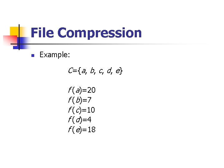
File Compression n Example: C={a, b, c, d, e} f (a)=20 f (b)=7 f (c)=10 f (d)=4 f (e)=18

The Greedy Approach n Other examples: Dijkstra’s algorithm for the shortest path problem Ø Kruskal’s algorithm for the minimum cost spanning tree problem Ø

Divide and Conquer n A divide-and-conquer algorithm divides the problem instance into a number of subinstances (in most cases 2), recursively solves each subinsance separately, and then combines the solutions to the subinstances to obtain the solution to the original problem instance.

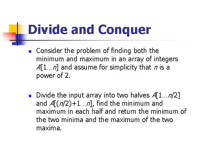
Divide and Conquer n n Consider the problem of finding both the minimum and maximum in an array of integers A[1…n] and assume for simplicity that n is a power of 2. Divide the input array into two halves A[1…n/2] and A[(n/2)+1…n], find the minimum and maximum in each half and return the minimum of the two minima and the maximum of the two maxima.

Divide and Conquer n n n n Input: An array A[1…n] of n integers, where n is a power of 2; Output: (x, y): the minimum and maximum integers in A; 1. minmax(1, n); minmax(low, high) 1. if high-low=1 then 2. if A[low]<A[high] then return (A[low], A[high]); 3. else return(A[high], A[low]); 4. end if; 5. else 6. mid (low+high)/2 ; 7. (x 1, y 1) minmax(low, mid); 8. (x 2, y 2) minmax(mid+1, high); 9. x min{x 1, x 2}; 10. y max{y 1, y 2}; 11. return(x, y); 12. end if;

Divide and Conquer n How many comparisons does this algorithm need?

Divide and Conquer n Given an array A[1…n] of n elements, where n is a power of 2, it is possible to find both the minimum and maximum of the elements in A using only (3 n/2)-2 element comparisons.

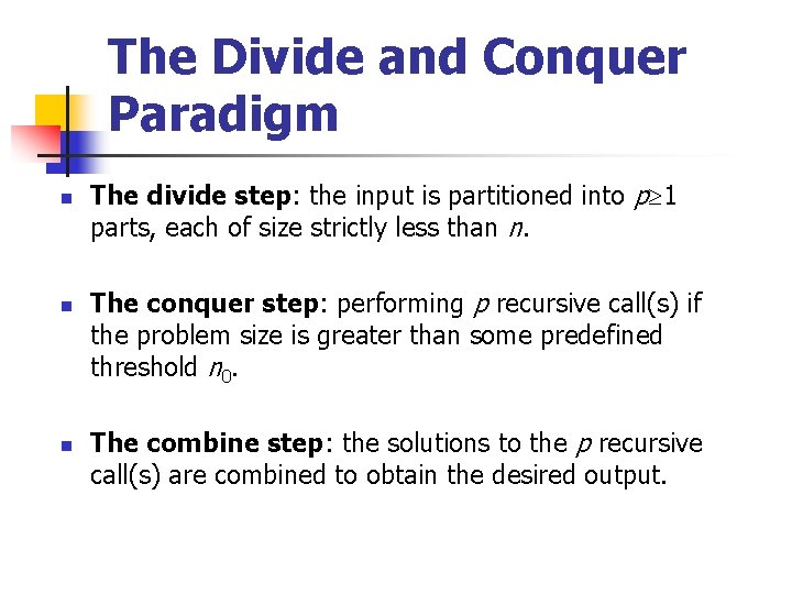
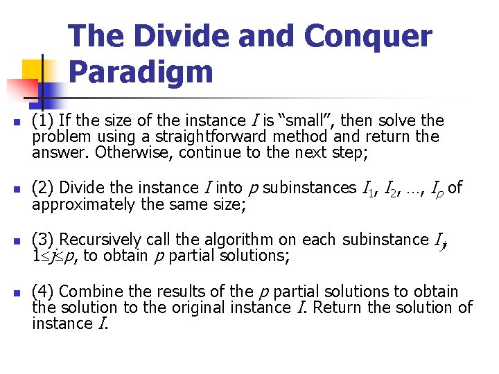
The Divide and Conquer Paradigm n n n The divide step: the input is partitioned into p 1 parts, each of size strictly less than n. The conquer step: performing p recursive call(s) if the problem size is greater than some predefined threshold n 0. The combine step: the solutions to the p recursive call(s) are combined to obtain the desired output.

The Divide and Conquer Paradigm n (1) If the size of the instance I is “small”, then solve the problem using a straightforward method and return the answer. Otherwise, continue to the next step; n (2) Divide the instance I into p subinstances I 1, I 2, …, Ip of approximately the same size; n (3) Recursively call the algorithm on each subinstance Ij, 1 j p, to obtain p partial solutions; n (4) Combine the results of the p partial solutions to obtain the solution to the original instance I. Return the solution of instance I.

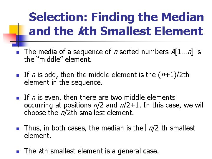
Selection: Finding the Median and the kth Smallest Element n n n The media of a sequence of n sorted numbers A[1…n] is the “middle” element. If n is odd, then the middle element is the (n+1)/2 th element in the sequence. If n is even, then there are two middle elements occurring at positions n/2 and n/2+1. In this case, we will choose the n/2 th smallest element. Thus, in both cases, the median is the n/2 th smallest element. The kth smallest element is a general case.

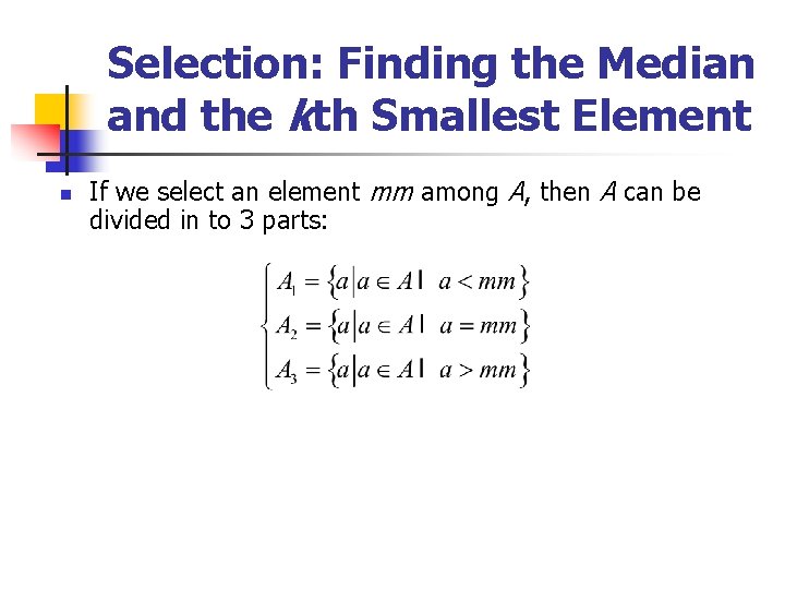
Selection: Finding the Median and the kth Smallest Element n If we select an element mm among A, then A can be divided in to 3 parts:

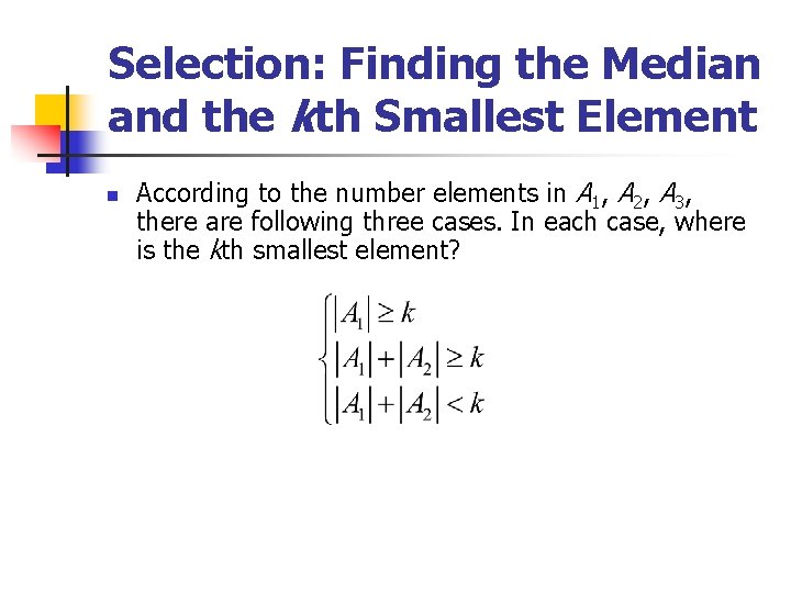
Selection: Finding the Median and the kth Smallest Element n According to the number elements in A 1, A 2, A 3, there are following three cases. In each case, where is the kth smallest element?

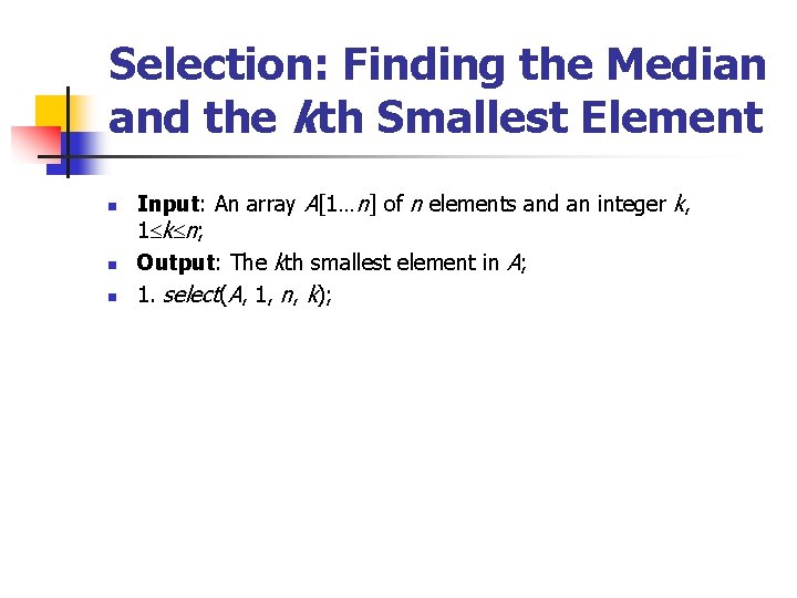
Selection: Finding the Median and the kth Smallest Element n n n Input: An array A[1…n] of n elements and an integer k, 1 k n; Output: The kth smallest element in A; 1. select(A, 1, n, k);

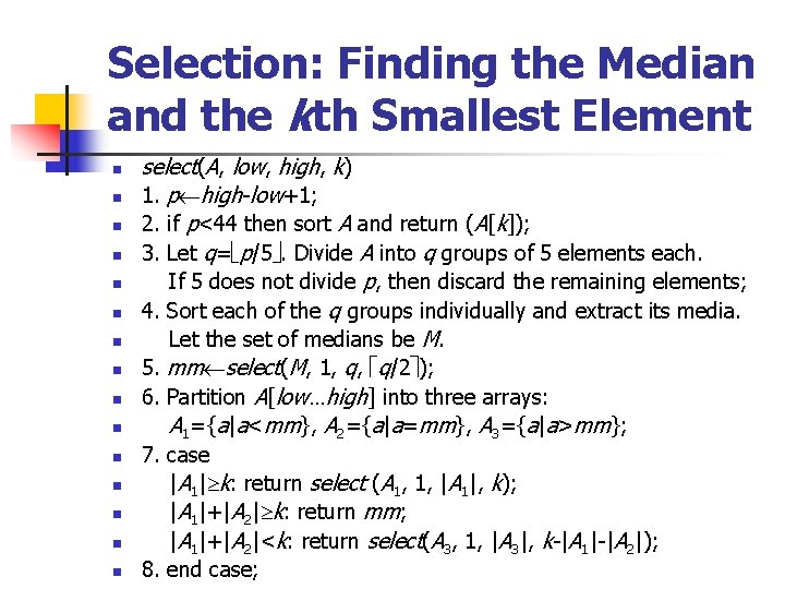
Selection: Finding the Median and the kth Smallest Element n n n n select(A, low, high, k) 1. p high-low+1; 2. if p<44 then sort A and return (A[k]); 3. Let q= p/5. Divide A into q groups of 5 elements each. If 5 does not divide p, then discard the remaining elements; 4. Sort each of the q groups individually and extract its media. Let the set of medians be M. 5. mm select(M, 1, q, q/2 ); 6. Partition A[low…high] into three arrays: A 1={a|a<mm}, A 2={a|a=mm}, A 3={a|a>mm}; 7. case |A 1| k: return select (A 1, 1, |A 1|, k); |A 1|+|A 2| k: return mm; |A 1|+|A 2|<k: return select(A 3, 1, |A 3|, k-|A 1|-|A 2|); 8. end case;

Selection: Finding the Median and the kth Smallest Element n What is the time complexity of this algorithm?

Selection: Finding the Median and the kth Smallest Element n The kth smallest element in a set of n elements drawn from a linearly ordered set can be found in (n) time.

Selection: Finding the Median and the kth Smallest Element n Write the codes for the above algorithm.

Divide and Conquer n Other example: Ø Quicksort

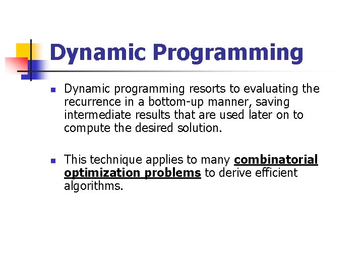
Dynamic Programming n n Dynamic programming resorts to evaluating the recurrence in a bottom-up manner, saving intermediate results that are used later on to compute the desired solution. This technique applies to many combinatorial optimization problems to derive efficient algorithms.

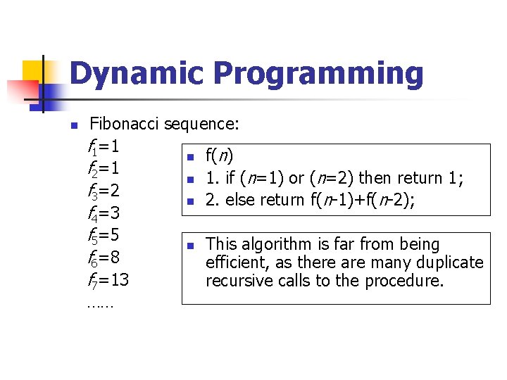
Dynamic Programming n Fibonacci sequence: f 1=1 n f(n) f 2=1 n 1. if (n=1) or (n=2) then return 1; f 3=2 n 2. else return f(n-1)+f(n-2); f 4=3 f 5=5 n This algorithm is far from being f 6=8 efficient, as there are many duplicate f 7=13 recursive calls to the procedure. ……

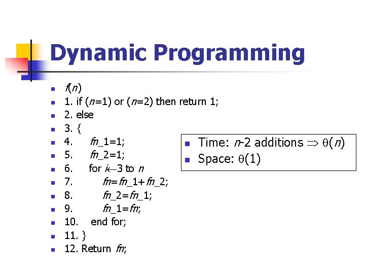
Dynamic Programming n n n n f( n ) 1. if (n=1) or (n=2) then return 1; 2. else 3. { 4. fn_1=1; n Time: n-2 additions 5. fn_2=1; n Space: (1) 6. for i 3 to n 7. fn=fn_1+fn_2; 8. fn_2=fn_1; 9. fn_1=fn; 10. end for; 11. } 12. Return fn; (n)

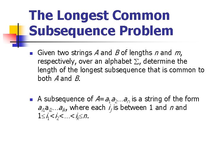
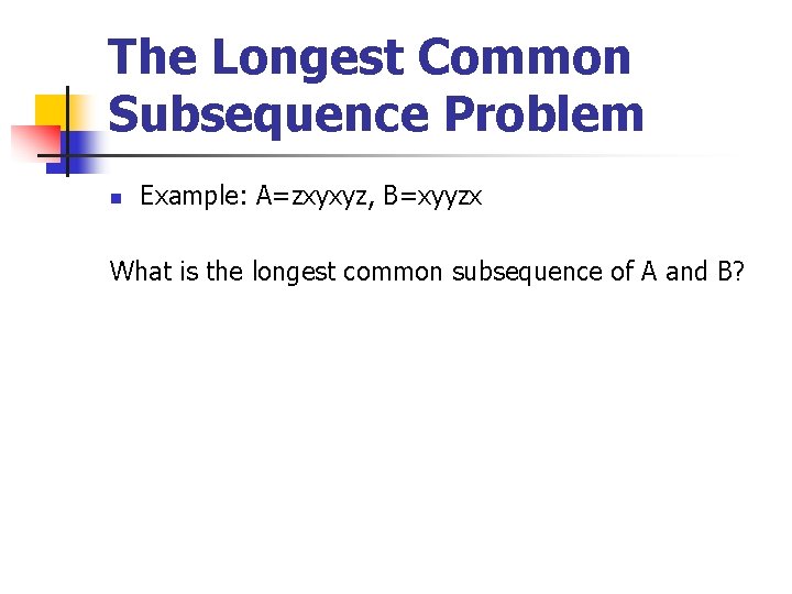
The Longest Common Subsequence Problem n n Given two strings A and B of lengths n and m, respectively, over an alphabet , determine the length of the longest subsequence that is common to both A and B. A subsequence of A=a 1 a 2…an is a string of the form ai 1 ai 2…aik, where each ij is between 1 and n and 1 i 1<i 2<…<ik n.

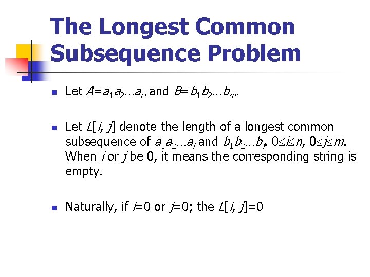
The Longest Common Subsequence Problem n n n Let A=a 1 a 2…an and B=b 1 b 2…bm. Let L[i, j] denote the length of a longest common subsequence of a 1 a 2…ai and b 1 b 2…bj. 0 i n, 0 j m. When i or j be 0, it means the corresponding string is empty. Naturally, if i=0 or j=0; the L[i, j]=0

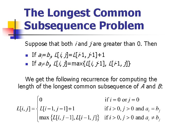
The Longest Common Subsequence Problem Suppose that both i and j are greater than 0. Then n n If ai=bj, L[i, j]=L[i-1, j-1]+1 If ai bj, L[i, j]=max{L[i, j-1], L[i-1, j]} We get the following recurrence for computing the length of the longest common subsequence of A and B:

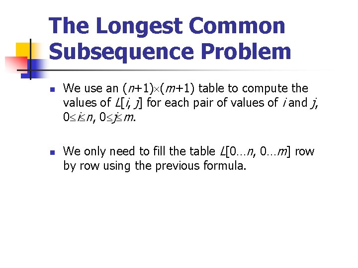
The Longest Common Subsequence Problem n n We use an (n+1) (m+1) table to compute the values of L[i, j] for each pair of values of i and j, 0 i n, 0 j m. We only need to fill the table L[0…n, 0…m] row by row using the previous formula.

The Longest Common Subsequence Problem n Example: A=zxyxyz, B=xyyzx What is the longest common subsequence of A and B?

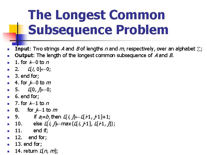
The Longest Common Subsequence Problem n n n n Input: Two strings A and B of lengths n and m, respectively, over an alphabet ; Output: The length of the longest common subsequence of A and B. 1. for i 0 to n 2. L[i, 0] 0; 3. end for; 4. for j 0 to m 5. L[0, j] 0; 6. end for; 7. for i 1 to n 8. for j 1 to m 9. if ai=bj then L[i, j] L[i-1, j-1]+1; 10. else L[i, j] max{L[i, j-1], L[i-1, j]}; 11. end if; 12. end for; 13. end for; 14. return L[n, m];

The Longest Common Subsequence Problem n What’s the performance of this algorithm? ü Time Complexity? ü Space Complexity?

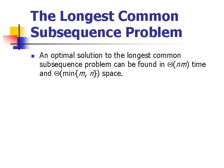
The Longest Common Subsequence Problem n An optimal solution to the longest common subsequence problem can be found in (nm) time and (min{m, n}) space.

The Dynamic Programming Paradigm n n The idea of saving solutions to subproblems in order to avoid their recomputation is the basis of this powerful method. This is usually the case in many combinatorial optimization problems in which the solution can be expressed in the form of a recurrence whose direct solution causes subinstances to be computed more than once.

The Dynamic Programming Paradigm n n An important observation about the working of dynamic programming is that the algorithm computes an optimal solution to every subinstance of the original instance considered by the algorithm. This argument illustrates an important principle in algorithm design called the principle of optimality: Given an optimal sequence of decisions, each subsequence must be an optimal sequence of decisions by itself.

The Knapsack Problem n n Let U={u 1, u 2, …, un} be a set of n items to be packed in a knapsack of size C. for 1 j n, let sj and vj be the size and value of the jth item, respectively, where C and sj, vj, 1 j n, are all positive integers. The objective is to fill the knapsack with some items for U whose total size is at most C and such that their total value is maximum. Assume without loss of generality that the size of each item does not exceed C.

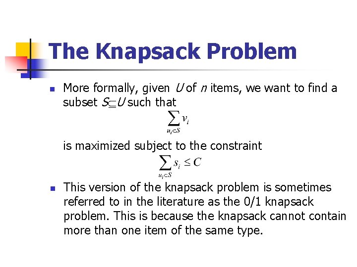
The Knapsack Problem n More formally, given U of n items, we want to find a subset S U such that is maximized subject to the constraint n This version of the knapsack problem is sometimes referred to in the literature as the 0/1 knapsack problem. This is because the knapsack cannot contain more than one item of the same type.

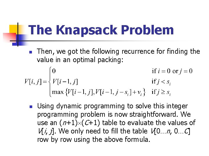
The Knapsack Problem n n Let V[i, j] denote the value obtained by filling a knapsack of size j with items taken from the first i items {u 1, u 2, …, ui} in an optimal way. Here the range of i is from 0 to n and the range of j is from 0 to C. Thus, what we seek is the value V[n, C]. Obviously, V[0, j] is 0 for all values of j, as there is nothing in the knapsack. On the other hand, V[i, 0] is 0 for all values of i since nothing can be put in a knapsack of size 0.

The Knapsack Problem n V[i, j], where i>0 and j>0, is the maximum of the following two quantities: ü V[i-1, j]: The maximum value obtained by filling a knapsack of size j with items taken from {u 1, u 2, …, ui -1} only in an optimal way. üV[i-1, j-si]+vi: The maximum value obtained by filling a knapsack of size j-si with items taken from {u 1, u 2, …, ui-1} in an optimal way plus the value of item ui. This case applies only if j si and it amounts to adding item ui to the knapsack.

The Knapsack Problem n n Then, we got the following recurrence for finding the value in an optimal packing: Using dynamic programming to solve this integer programming problem is now straightforward. We use an (n+1) (C+1) table to evaluate the values of V[i, j]. We only need to fill the table V[0…n, 0…C] row by row using the above formula.

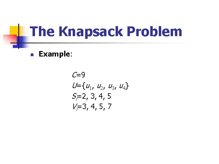
The Knapsack Problem n Example: C=9 U={u 1, u 2, u 3, u 4} Si=2, 3, 4, 5 Vi=3, 4, 5, 7

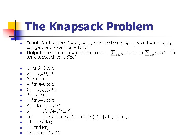
The Knapsack Problem n n n n Input: A set of items U={u 1, u 2, …, un} with sizes s 1, s 2, …, sn and values v 1, v 2, …, vn and a knapsack capacity C. Output: The maximum value of the function subject to for some subset of items S U. 1. for i 0 to n 2. V[i, 0] 0; 3. end for; 4. for j 0 to C 5. V[0, j] 0; 6. end for; 7. for i 1 to n 8. for j 1 to C 9. V[i, j] V[i-1, j]; 10. if si j then V[i, j] max{V[i, j], V[i-1, j-si]+vi}; 11. end for; 12. end for; 13. return V[n, C];

The Knapsack Problem n What is the time and space complexity of this algorithm?

The Knapsack Problem n An optimal solution to the Knapsack problem can be found in (n. C) time and (C) space.

Dynamic Programming n Other example: Ø Floyd Algorithm for the All-Pairs Shortest Path Problem

Backtracking n n In many real world problems, a solution can be obtained by exhaustively searching through a large but finite number of possibilities. Hence, the need arose for developing systematic techniques of searching, with the hope of cutting down the search space to possibly a much smaller space. Here, we present a general technique for organizing the search known as backtracking. This algorithm design technique can be described as an organized exhaustive search which often avoids searching all possibilities.

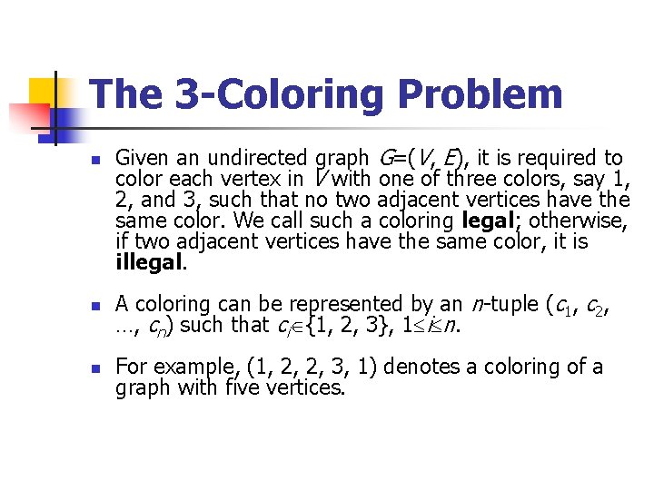
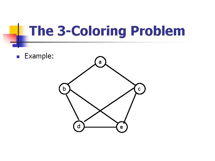
The 3 -Coloring Problem n n n Given an undirected graph G=(V, E), it is required to color each vertex in V with one of three colors, say 1, 2, and 3, such that no two adjacent vertices have the same color. We call such a coloring legal; otherwise, if two adjacent vertices have the same color, it is illegal. A coloring can be represented by an n-tuple (c 1, c 2, …, cn) such that ci {1, 2, 3}, 1 i n. For example, (1, 2, 2, 3, 1) denotes a coloring of a graph with five vertices.

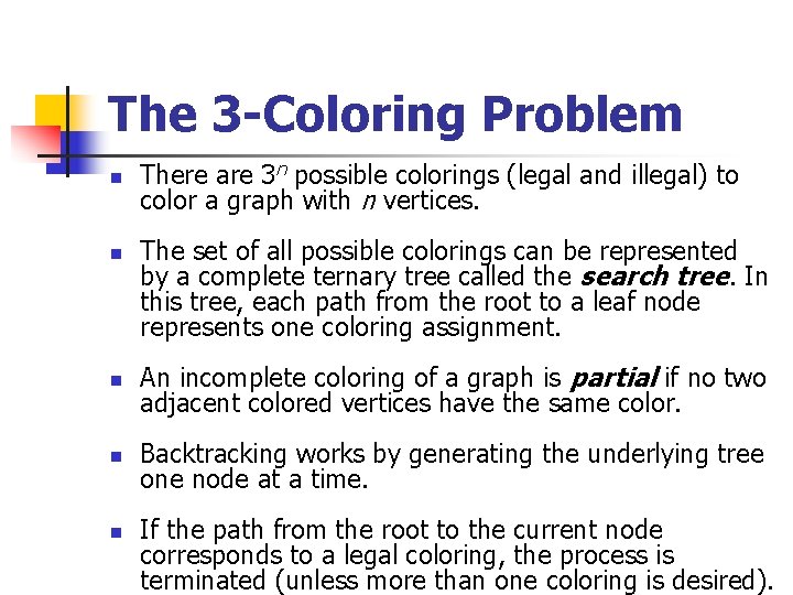
The 3 -Coloring Problem n n There are 3 n possible colorings (legal and illegal) to color a graph with n vertices. The set of all possible colorings can be represented by a complete ternary tree called the search tree. In this tree, each path from the root to a leaf node represents one coloring assignment. n An incomplete coloring of a graph is partial if no two adjacent colored vertices have the same color. n Backtracking works by generating the underlying tree one node at a time. n If the path from the root to the current node corresponds to a legal coloring, the process is terminated (unless more than one coloring is desired).

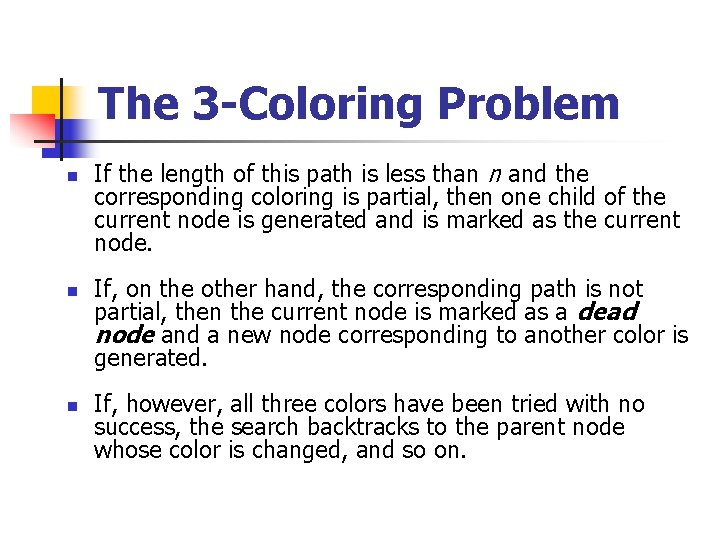
The 3 -Coloring Problem n n n If the length of this path is less than n and the corresponding coloring is partial, then one child of the current node is generated and is marked as the current node. If, on the other hand, the corresponding path is not partial, then the current node is marked as a dead node and a new node corresponding to another color is generated. If, however, all three colors have been tried with no success, the search backtracks to the parent node whose color is changed, and so on.

The 3 -Coloring Problem n Example: a b c d e

The 3 -Coloring Problem There are two important observations to be noted, which generalize to all backtracking algorithms: (1) The nodes are generated in a depth-first-search manner. (2) There is no need to store the whole search tree; we only need to store the path from the root to the current active node. In fact, no physical nodes are generated at all; the whole tree is implicit. We only need to keep track of the color assignment.

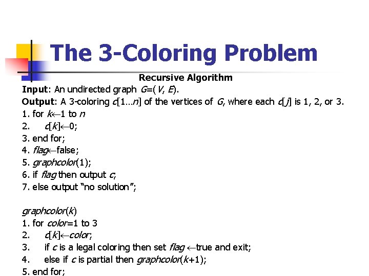
The 3 -Coloring Problem Recursive Algorithm Input: An undirected graph G=(V, E). Output: A 3 -coloring c[1…n] of the vertices of G, where each c[j] is 1, 2, or 3. 1. for k 1 to n 2. c[k] 0; 3. end for; 4. flag false; 5. graphcolor(1); 6. if flag then output c; 7. else output “no solution”; graphcolor(k) 1. for color=1 to 3 2. c[k] color; 3. if c is a legal coloring then set flag true and exit; 4. else if c is partial then graphcolor(k+1); 5. end for;

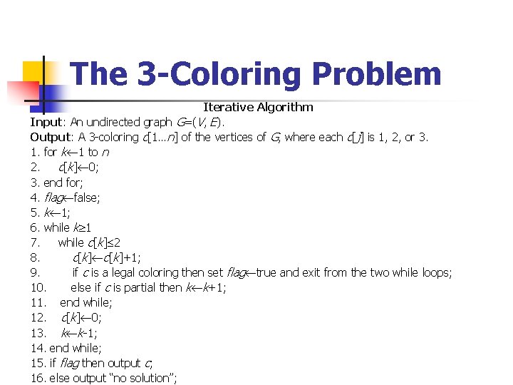
The 3 -Coloring Problem Iterative Algorithm Input: An undirected graph G=(V, E). Output: A 3 -coloring c[1…n] of the vertices of G, where each c[j] is 1, 2, or 3. 1. for k 1 to n 2. c[k] 0; 3. end for; 4. flag false; 5. k 1; 6. while k 1 7. while c[k] 2 8. c[k]+1; 9. if c is a legal coloring then set flag true and exit from the two while loops; 10. else if c is partial then k k+1; 11. end while; 12. c[k] 0; 13. k k-1; 14. end while; 15. if flag then output c; 16. else output “no solution”;

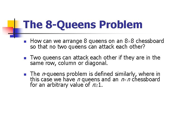
The 8 -Queens Problem n How can we arrange 8 queens on an 8 8 chessboard so that no two queens can attack each other? n Two queens can attack each other if they are in the same row, column or diagonal. n The n-queens problem is defined similarly, where in this case we have n queens and an n n chessboard for an arbitrary value of n 1.

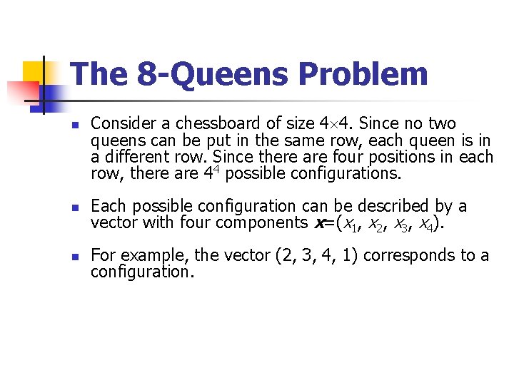
The 8 -Queens Problem n n n Consider a chessboard of size 4 4. Since no two queens can be put in the same row, each queen is in a different row. Since there are four positions in each row, there are 44 possible configurations. Each possible configuration can be described by a vector with four components x=(x 1, x 2, x 3, x 4). For example, the vector (2, 3, 4, 1) corresponds to a configuration.

The 8 -Queens Problem Input: none; n Output: A vector x[1… 4] corresponding to the solution of the 4 -queens problem. 1. for k 1 to 4 2. x[k] 0; 3. end for; 4. flag false; 5. k 1; 6. while k 1 7. while x[k] 3 8. x[k]+1; 9. if x is a legal placement then set flag true and exit from the two while loops; 10. else if x is partial then k k+1; 11. end while; 12. x[k] 0; 13. k k-1; 14. end while; 15. if flag then output x; 16. else output “no solution”; n

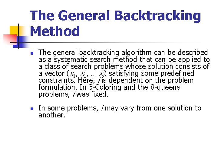
The General Backtracking Method n n The general backtracking algorithm can be described as a systematic search method that can be applied to a class of search problems whose solution consists of a vector (x 1, x 2, … xi) satisfying some predefined constraints. Here, i is dependent on the problem formulation. In 3 -Coloring and the 8 -queens problems, i was fixed. In some problems, i may vary from one solution to another.

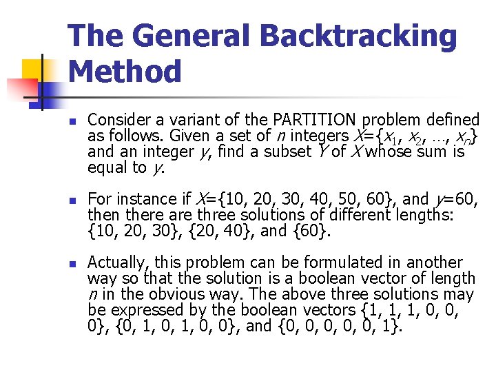
The General Backtracking Method n n n Consider a variant of the PARTITION problem defined as follows. Given a set of n integers X={x 1, x 2, …, xn} and an integer y, find a subset Y of X whose sum is equal to y. For instance if X={10, 20, 30, 40, 50, 60}, and y=60, then there are three solutions of different lengths: {10, 20, 30}, {20, 40}, and {60}. Actually, this problem can be formulated in another way so that the solution is a boolean vector of length n in the obvious way. The above three solutions may be expressed by the boolean vectors {1, 1, 1, 0, 0, 0}, {0, 1, 0, 0}, and {0, 0, 0, 1}.

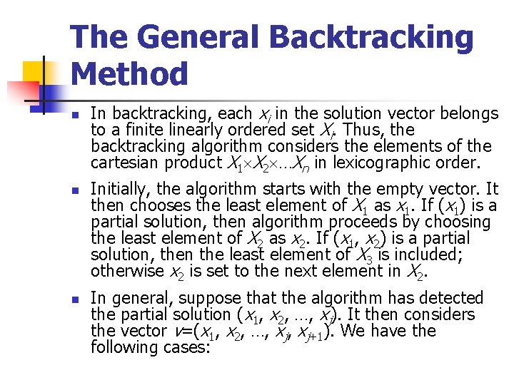
The General Backtracking Method n n n In backtracking, each xi in the solution vector belongs to a finite linearly ordered set Xi. Thus, the backtracking algorithm considers the elements of the cartesian product X 1 X 2 …Xn in lexicographic order. Initially, the algorithm starts with the empty vector. It then chooses the least element of X 1 as x 1. If (x 1) is a partial solution, then algorithm proceeds by choosing the least element of X 2 as x 2. If (x 1, x 2) is a partial solution, then the least element of X 3 is included; otherwise x 2 is set to the next element in X 2. In general, suppose that the algorithm has detected the partial solution (x 1, x 2, …, xj). It then considers the vector v=(x 1, x 2, …, xj+1). We have the following cases:

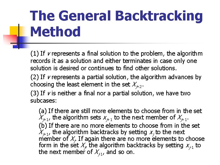
The General Backtracking Method (1) If v represents a final solution to the problem, the algorithm records it as a solution and either terminates in case only one solution is desired or continues to find other solutions. (2) If v represents a partial solution, the algorithm advances by choosing the least element in the set Xj+2. (3) If v is neither a final nor a partial solution, we have two subcases: (a) If there are still more elements to choose from in the set Xj+1, the algorithm sets xj+1 to the next member of Xj+1. (b) If there are no more elements to choose from in the set Xj+1, the algorithm backtracks by setting xj to the next member of Xj. If again there are no more elements to choose form in the set Xj, the algorithm backtracks by setting xj-1 to the next member of Xj-1, and so on.

Homework 10. 3 10. 7 10. 54 10. 58 b