Data Flow Analysis Compiler Structure Source code parsed

Data Flow Analysis

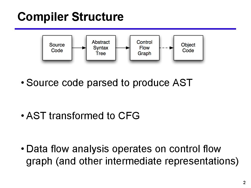
Compiler Structure • Source code parsed to produce AST • AST transformed to CFG • Data flow analysis operates on control flow graph (and other intermediate representations) 2

ASTs • ASTs are abstract ■ They don’t contain all information in the program - E. g. , spacing, comments, brackets, parentheses ■ Any ambiguity has been resolved - E. g. , a + b + c produces the same AST as (a + b) + c 3

Disadvantages of ASTs • AST has many similar forms ■ E. g. , for, while, repeat. . . until ■ E. g. , if, ? : , switch • Expressions in AST may be complex, nested ■ (42 * y) + (z > 5 ? 12 * z : z + 20) • Want simpler representation for analysis ■. . . at least, for dataflow analysis 4

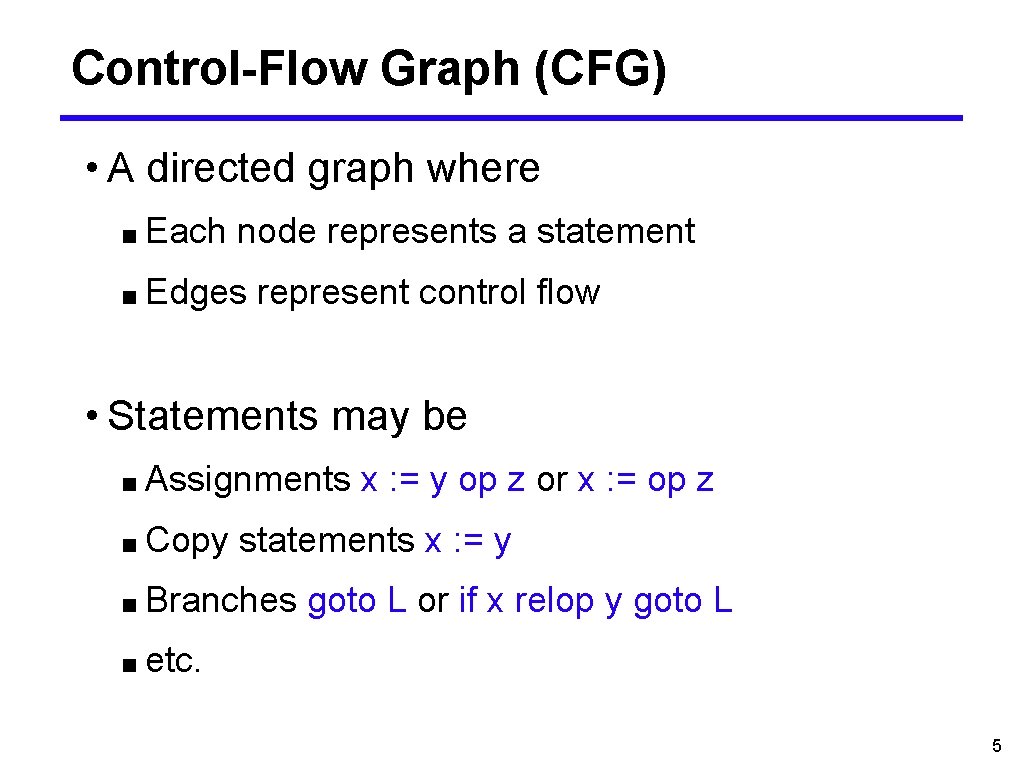
Control-Flow Graph (CFG) • A directed graph where ■ Each node represents a statement ■ Edges represent control flow • Statements may be ■ Assignments ■ Copy x : = y op z or x : = op z statements x : = y ■ Branches goto L or if x relop y goto L ■ etc. 5

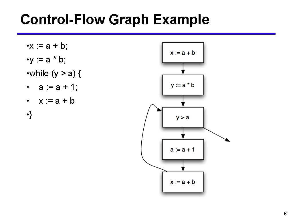
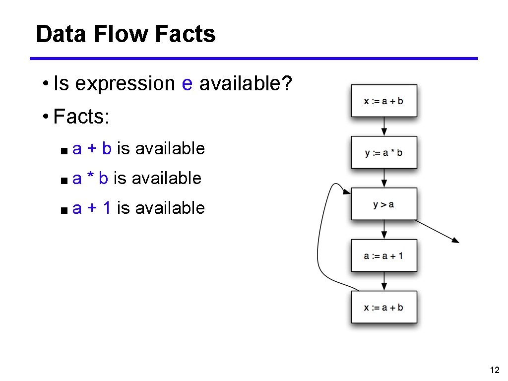
Control-Flow Graph Example • x : = a + b; • y : = a * b; • while (y > a) { • a : = a + 1; • x : = a + b • } 6

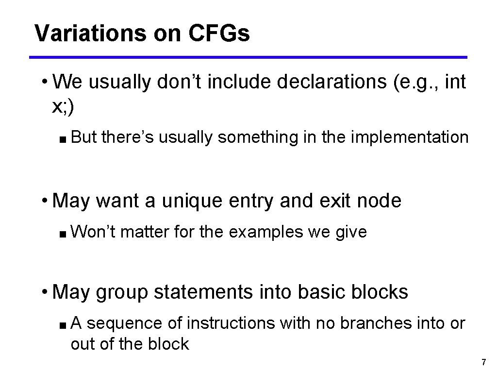
Variations on CFGs • We usually don’t include declarations (e. g. , int x; ) ■ But there’s usually something in the implementation • May want a unique entry and exit node ■ Won’t matter for the examples we give • May group statements into basic blocks ■A sequence of instructions with no branches into or out of the block 7

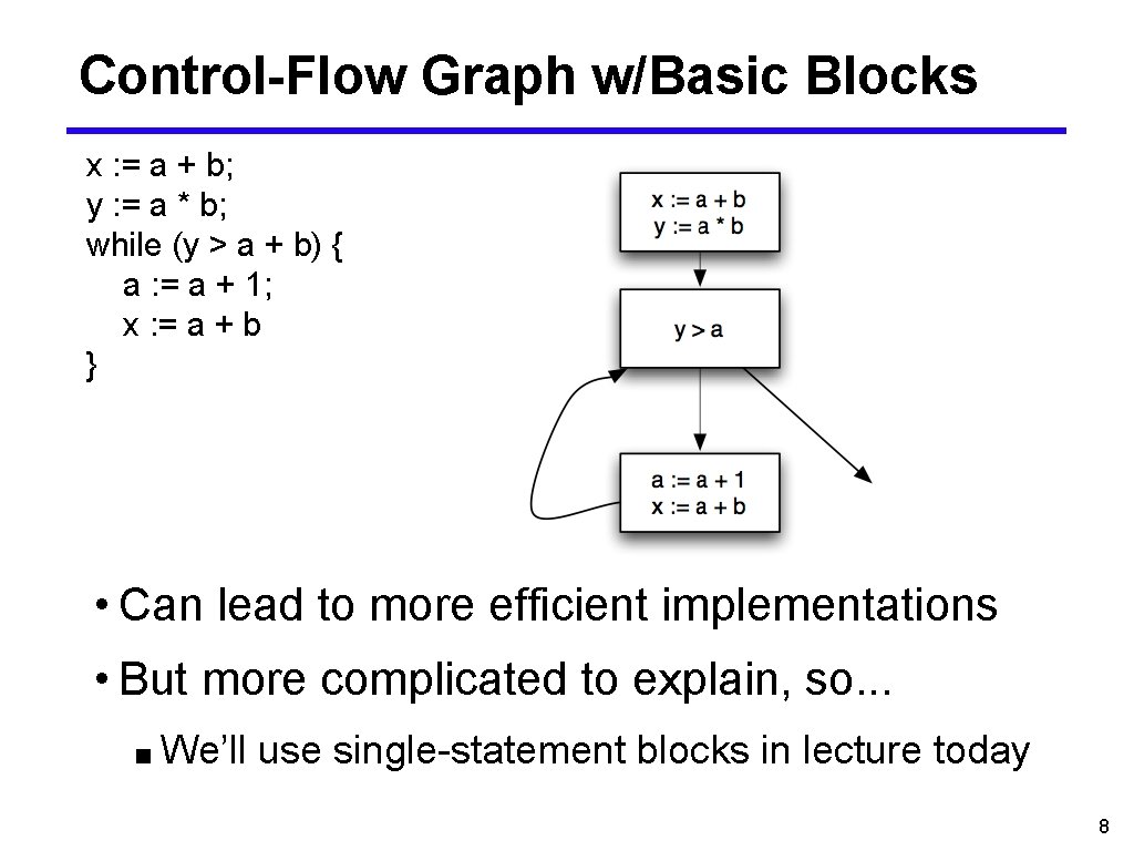
Control-Flow Graph w/Basic Blocks x : = a + b; y : = a * b; while (y > a + b) { a : = a + 1; x : = a + b } • Can lead to more efficient implementations • But more complicated to explain, so. . . ■ We’ll use single-statement blocks in lecture today 8

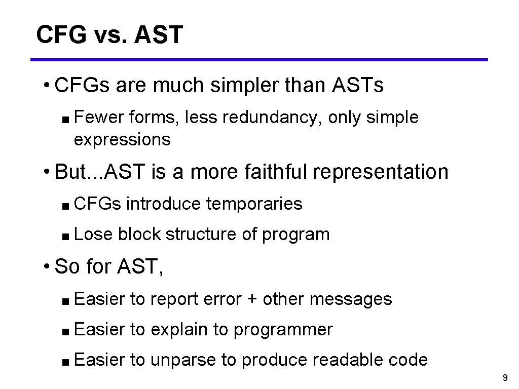
CFG vs. AST • CFGs are much simpler than ASTs ■ Fewer forms, less redundancy, only simple expressions • But. . . AST is a more faithful representation ■ CFGs ■ Lose introduce temporaries block structure of program • So for AST, ■ Easier to report error + other messages ■ Easier to explain to programmer ■ Easier to unparse to produce readable code 9

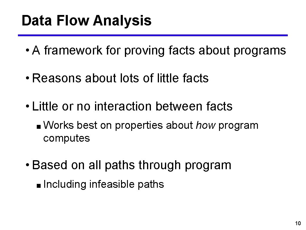
Data Flow Analysis • A framework for proving facts about programs • Reasons about lots of little facts • Little or no interaction between facts ■ Works best on properties about how program computes • Based on all paths through program ■ Including infeasible paths 10

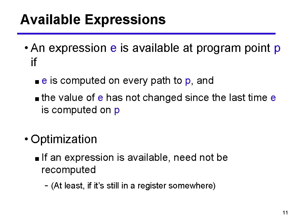
Available Expressions • An expression e is available at program point p if ■e is computed on every path to p, and ■ the value of e has not changed since the last time e is computed on p • Optimization ■ If an expression is available, need not be recomputed - (At least, if it’s still in a register somewhere) 11

Data Flow Facts • Is expression e available? • Facts: ■a + b is available ■a * b is available ■a + 1 is available 12

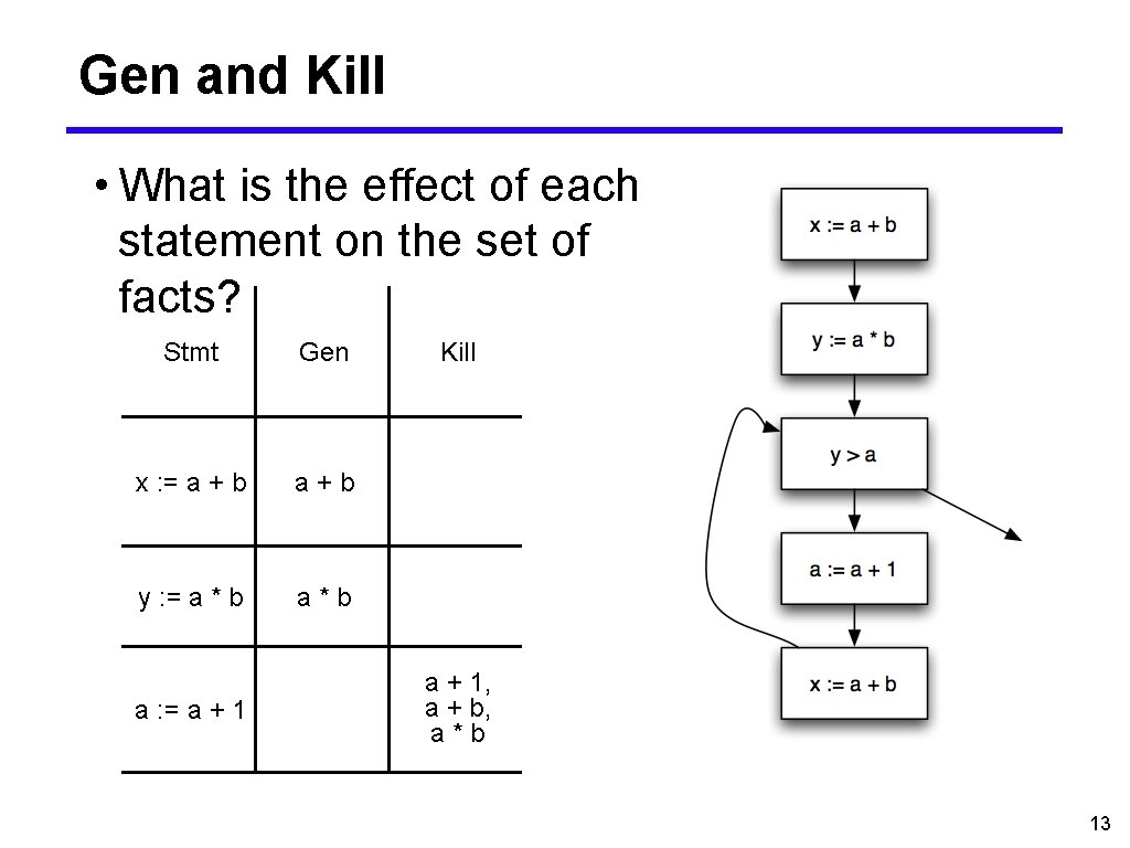
Gen and Kill • What is the effect of each statement on the set of facts? Stmt Gen x : = a + b a+b y : = a * b a*b a : = a + 1 Kill a + 1, a + b, a*b 13

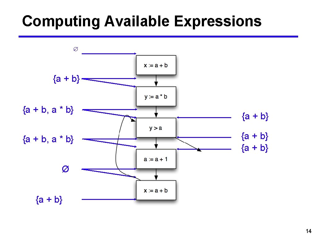
Computing Available Expressions ∅ {a + b} {a + b, a * b} {a + b} Ø {a + b} 14

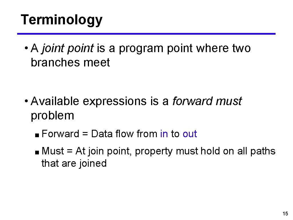
Terminology • A joint point is a program point where two branches meet • Available expressions is a forward must problem ■ Forward = Data flow from in to out ■ Must = At join point, property must hold on all paths that are joined 15

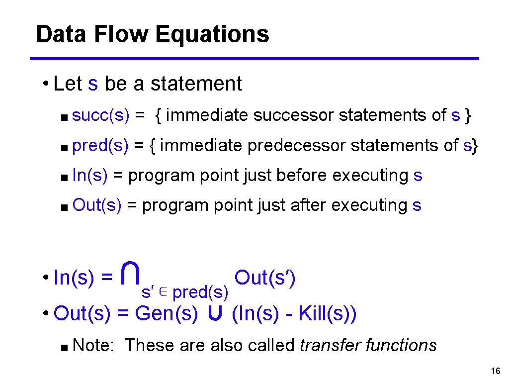
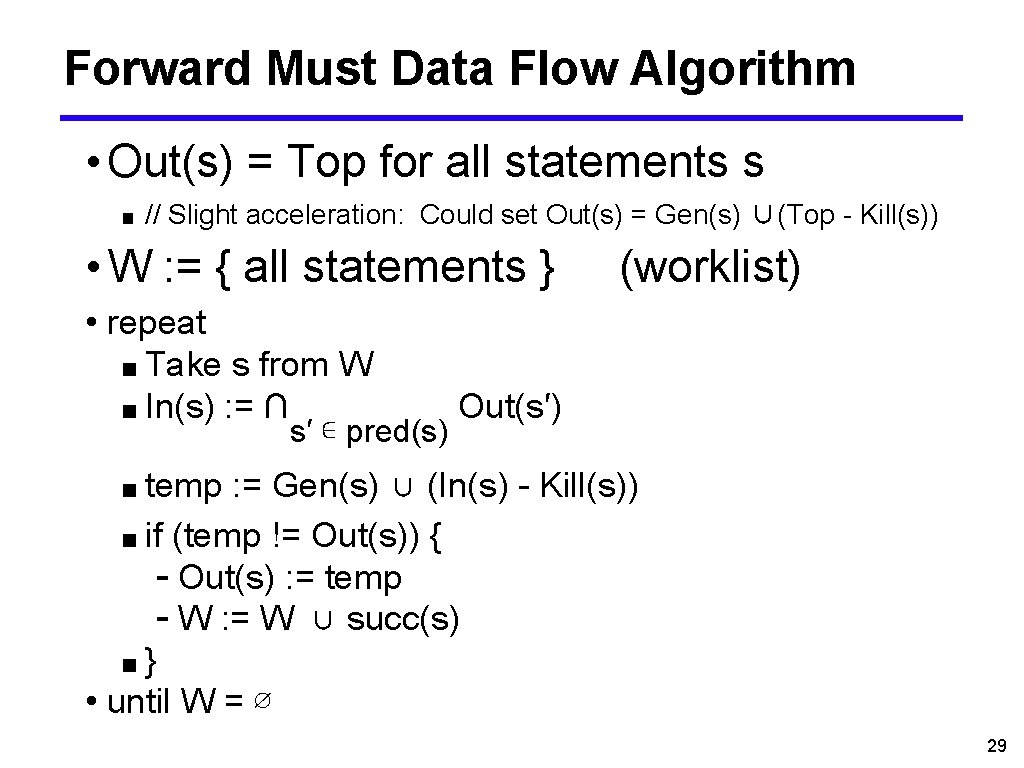
Data Flow Equations • Let s be a statement ■ succ(s) = { immediate successor statements of s } ■ pred(s) = { immediate predecessor statements of s} ■ In(s) = program point just before executing s ■ Out(s) = program point just after executing s • In(s) = ∩ s′ ∊ pred(s) Out(s′) • Out(s) = Gen(s) ∪ (In(s) - Kill(s)) ■ Note: These are also called transfer functions 16

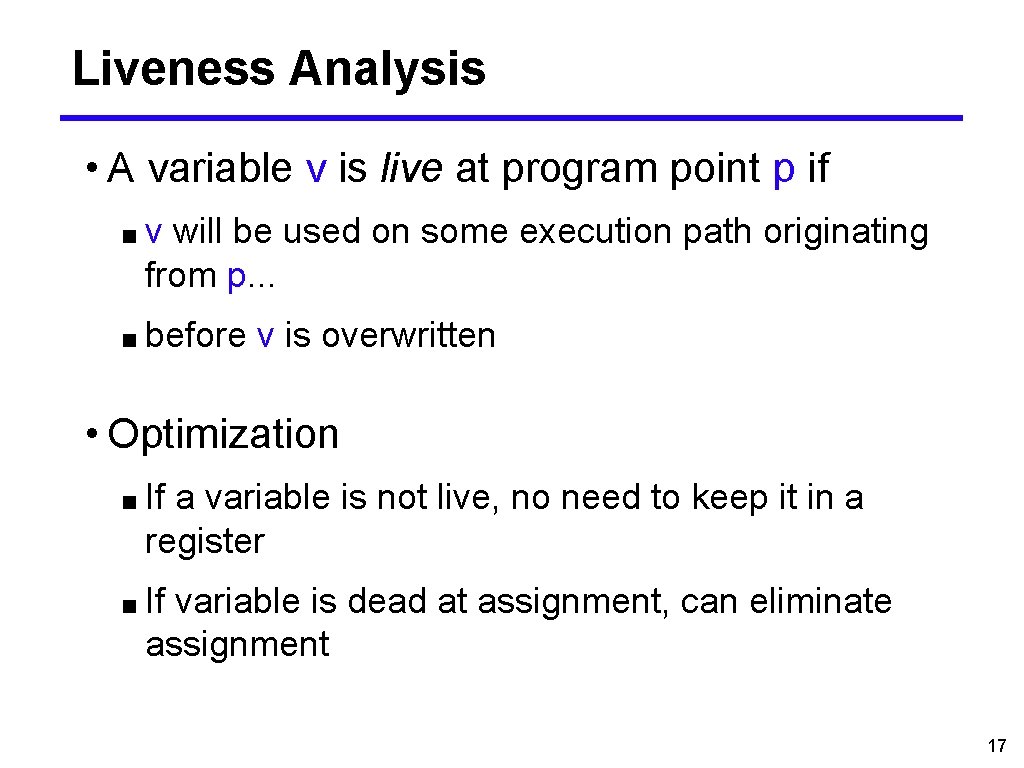
Liveness Analysis • A variable v is live at program point p if ■v will be used on some execution path originating from p. . . ■ before v is overwritten • Optimization ■ If a variable is not live, no need to keep it in a register ■ If variable is dead at assignment, can eliminate assignment 17

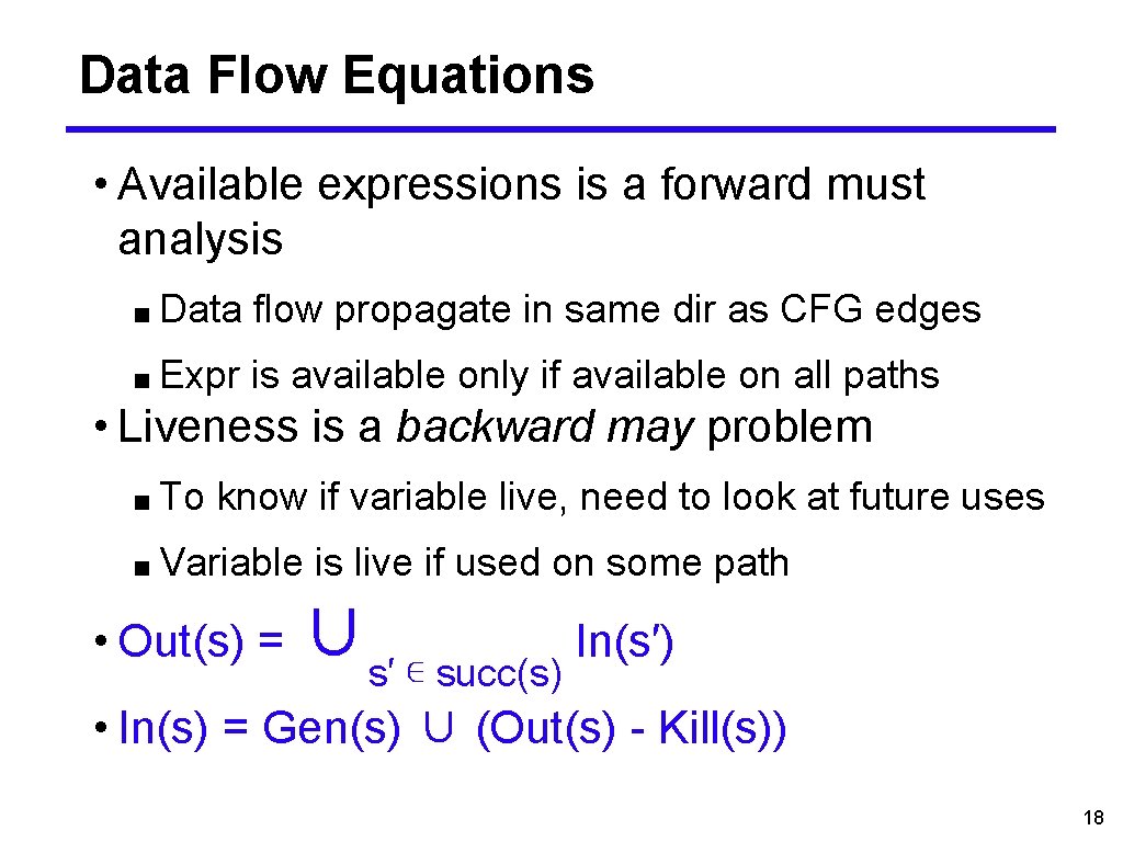
Data Flow Equations • Available expressions is a forward must analysis ■ Data flow propagate in same dir as CFG edges ■ Expr is available only if available on all paths • Liveness is a backward may problem ■ To know if variable live, need to look at future uses ■ Variable is live if used on some path • Out(s) = ∪ s′ ∊ succ(s) In(s′) • In(s) = Gen(s) ∪ (Out(s) - Kill(s)) 18

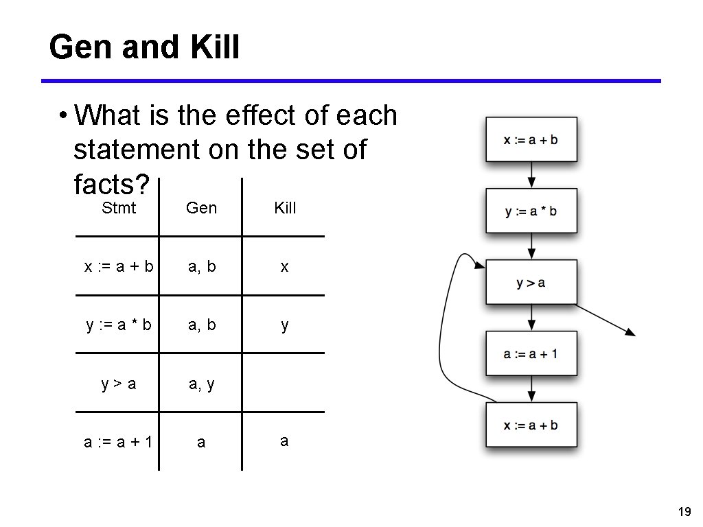
Gen and Kill • What is the effect of each statement on the set of facts? Stmt Gen Kill x : = a + b a, b x y : = a * b a, b y y>a a, y a : = a + 1 a a 19

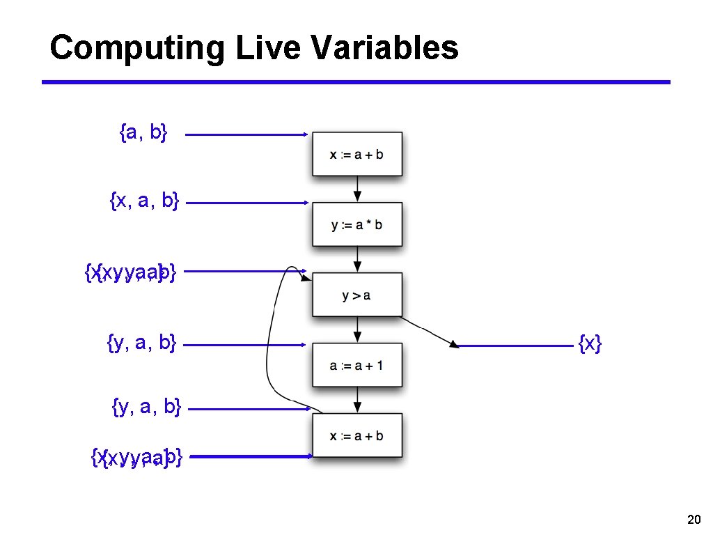
Computing Live Variables {a, b} {x, {x, y, y, a, a}b} {y, a, b} {x, {x, y, y, a, a}b} 20

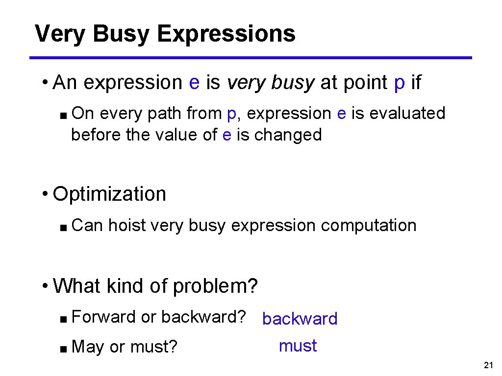
Very Busy Expressions • An expression e is very busy at point p if ■ On every path from p, expression e is evaluated before the value of e is changed • Optimization ■ Can hoist very busy expression computation • What kind of problem? ■ Forward ■ May or backward? backward or must? must 21

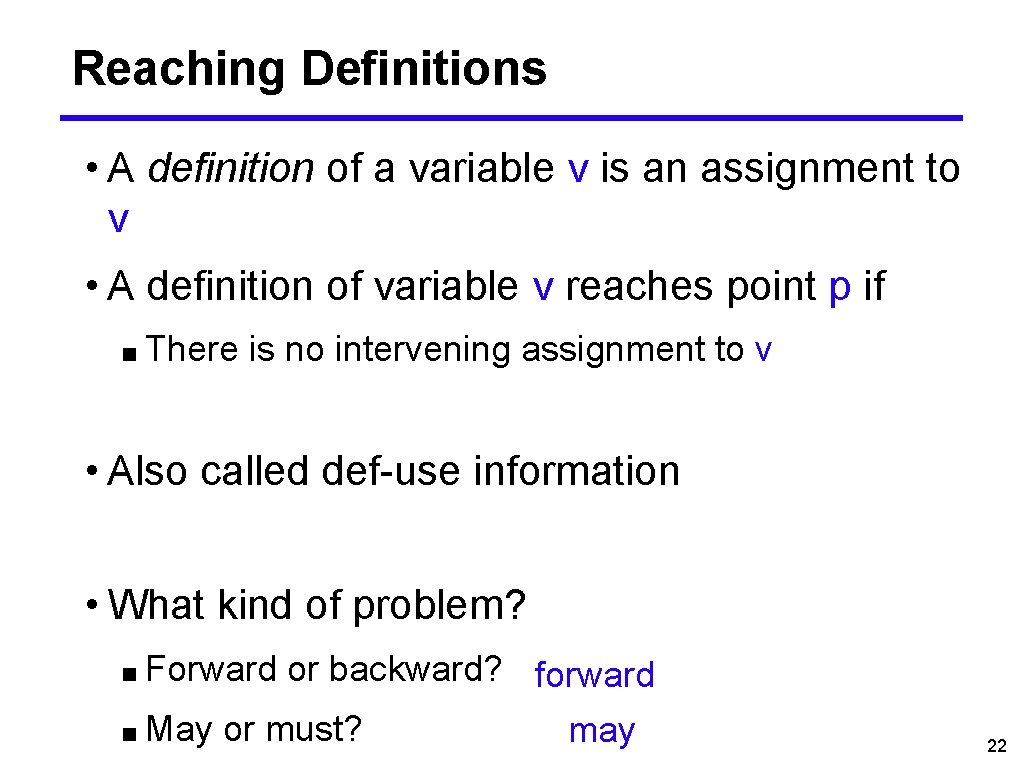
Reaching Definitions • A definition of a variable v is an assignment to v • A definition of variable v reaches point p if ■ There is no intervening assignment to v • Also called def-use information • What kind of problem? ■ Forward ■ May or backward? forward or must? may 22

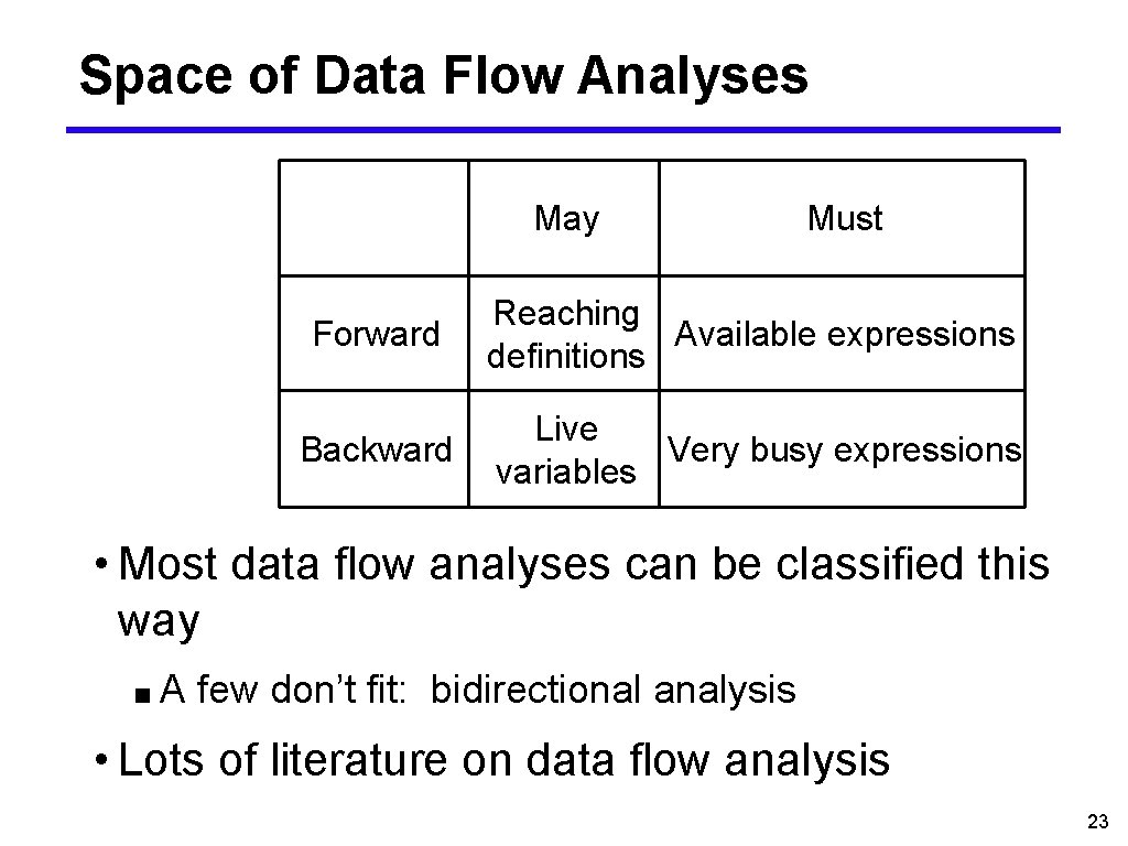
Space of Data Flow Analyses May Must Forward Reaching Available expressions definitions Backward Live Very busy expressions variables • Most data flow analyses can be classified this way ■A few don’t fit: bidirectional analysis • Lots of literature on data flow analysis 23

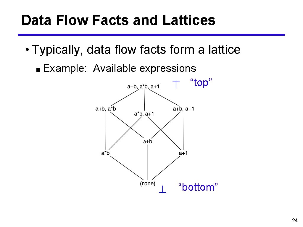
Data Flow Facts and Lattices • Typically, data flow facts form a lattice ■ Example: Available expressions “top” “bottom” 24

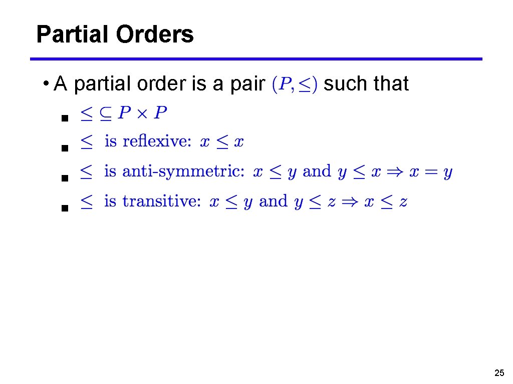
Partial Orders • A partial order is a pair such that ■ ■ 25

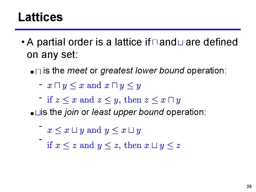
Lattices • A partial order is a lattice if and are defined on any set: is the meet or greatest lower bound operation: ■ ■ is the join or least upper bound operation: - 26

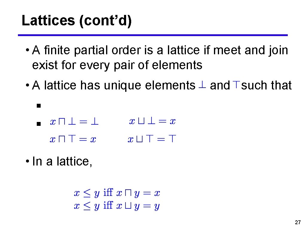
Lattices (cont’d) • A finite partial order is a lattice if meet and join exist for every pair of elements • A lattice has unique elements and such that ■ ■ • In a lattice, 27

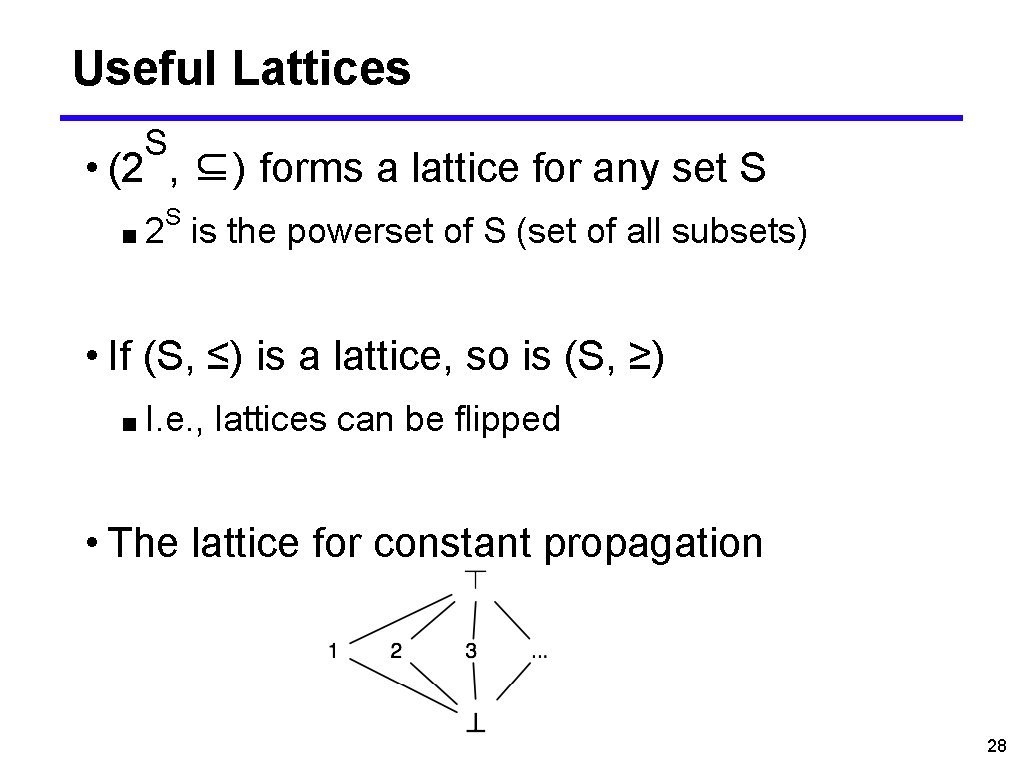
Useful Lattices S • (2 , ⊆) forms a lattice for any set S ■ 2 S is the powerset of S (set of all subsets) • If (S, ≤) is a lattice, so is (S, ≥) ■ I. e. , lattices can be flipped • The lattice for constant propagation 28

Forward Must Data Flow Algorithm • Out(s) = Top for all statements s ■ // Slight acceleration: Could set Out(s) = Gen(s) ∪(Top - Kill(s)) • W : = { all statements } • repeat ■ Take s from W ■ In(s) : = ∩ s′ ∊ pred(s) (worklist) Out(s′) ■ temp : = Gen(s) ∪ (In(s) - Kill(s)) ■ if (temp != Out(s)) { - Out(s) : = temp - W : = W ∪ succ(s) ■} • until W = ∅ 29

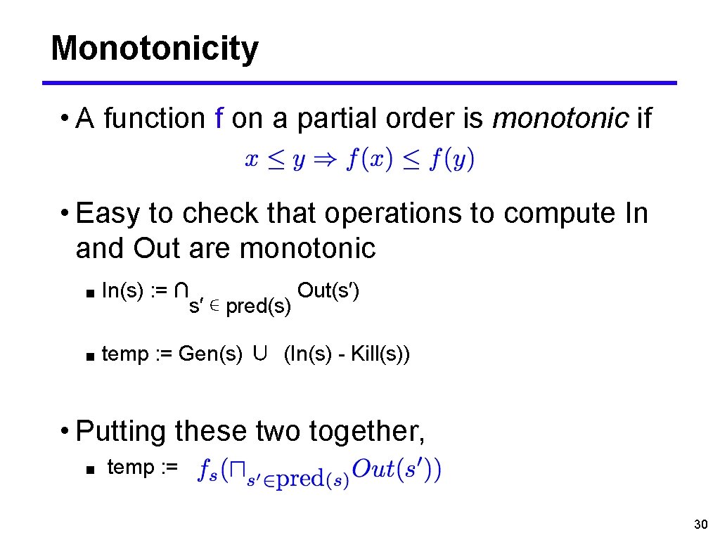
Monotonicity • A function f on a partial order is monotonic if • Easy to check that operations to compute In and Out are monotonic ■ In(s) : = ∩ ■ temp : = Gen(s) ∪ (In(s) - Kill(s)) s′ ∊ pred(s) Out(s′) • Putting these two together, ■ temp : = 30

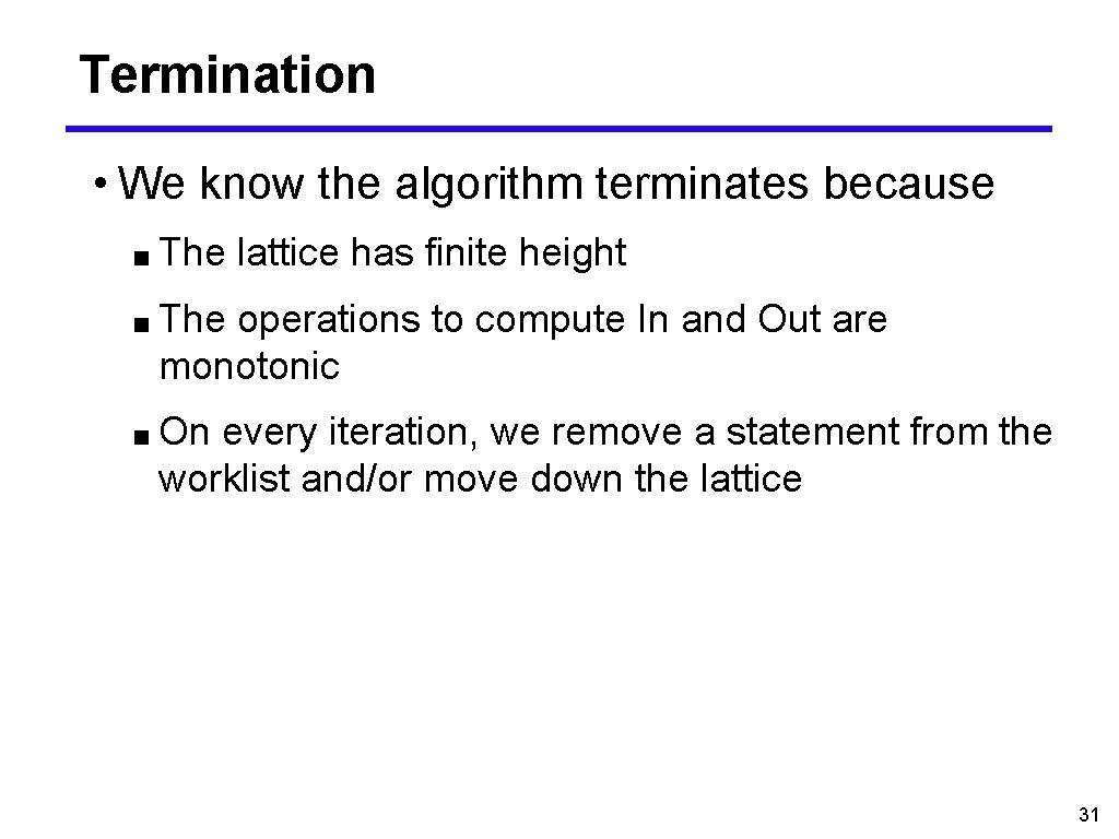
Termination • We know the algorithm terminates because ■ The lattice has finite height ■ The operations to compute In and Out are monotonic ■ On every iteration, we remove a statement from the worklist and/or move down the lattice 31

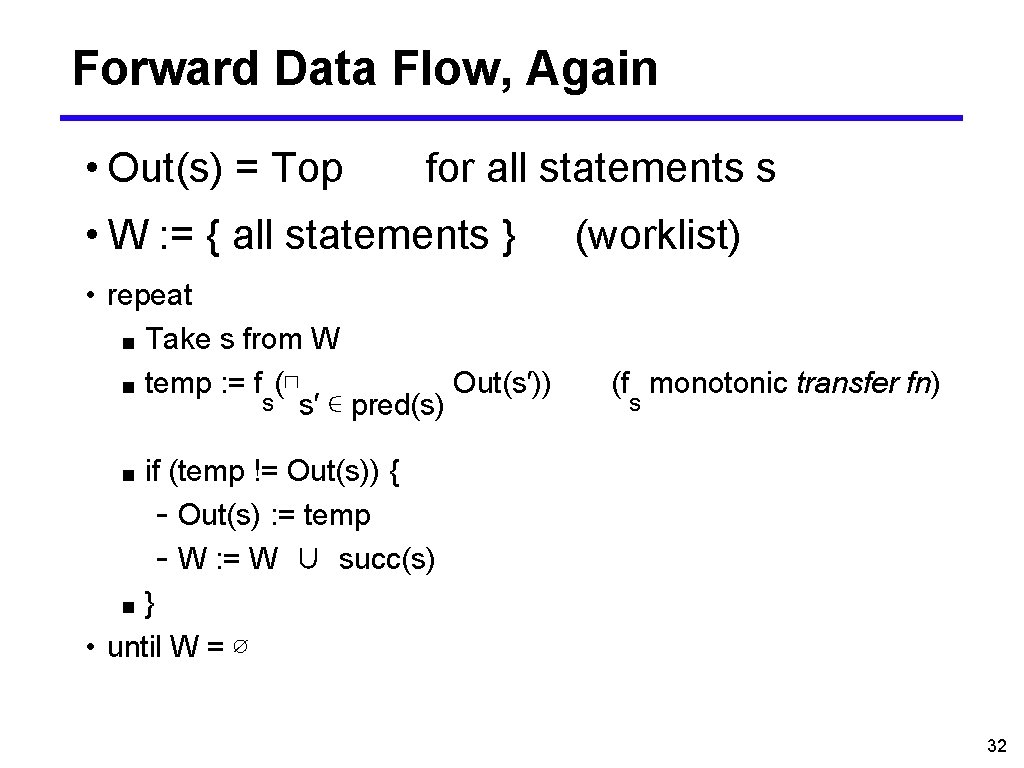
Forward Data Flow, Again • Out(s) = Top for all statements s • W : = { all statements } • repeat ■ Take s from W ■ temp : = f (⊓ Out(s′)) s s′ ∊ pred(s) (worklist) (f monotonic transfer fn) s if (temp != Out(s)) { - Out(s) : = temp - W : = W ∪ succ(s) ■} • until W = ∅ ■ 32

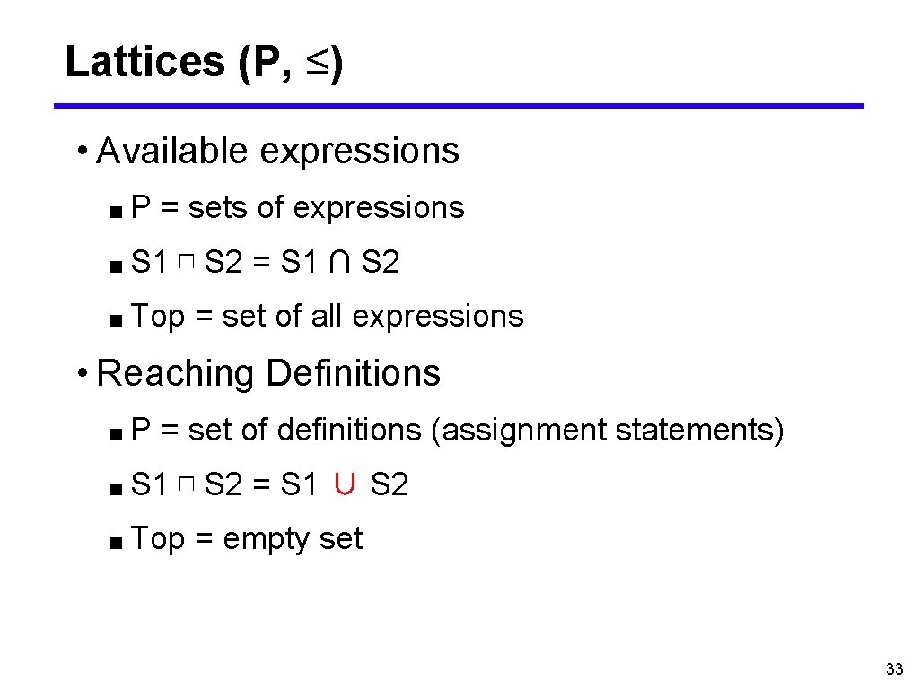
Lattices (P, ≤) • Available expressions ■P = sets of expressions ■ S 1 ⊓ S 2 = S 1 ∩ S 2 ■ Top = set of all expressions • Reaching Definitions ■P = set of definitions (assignment statements) ■ S 1 ⊓ S 2 = S 1 ∪ S 2 ■ Top = empty set 33

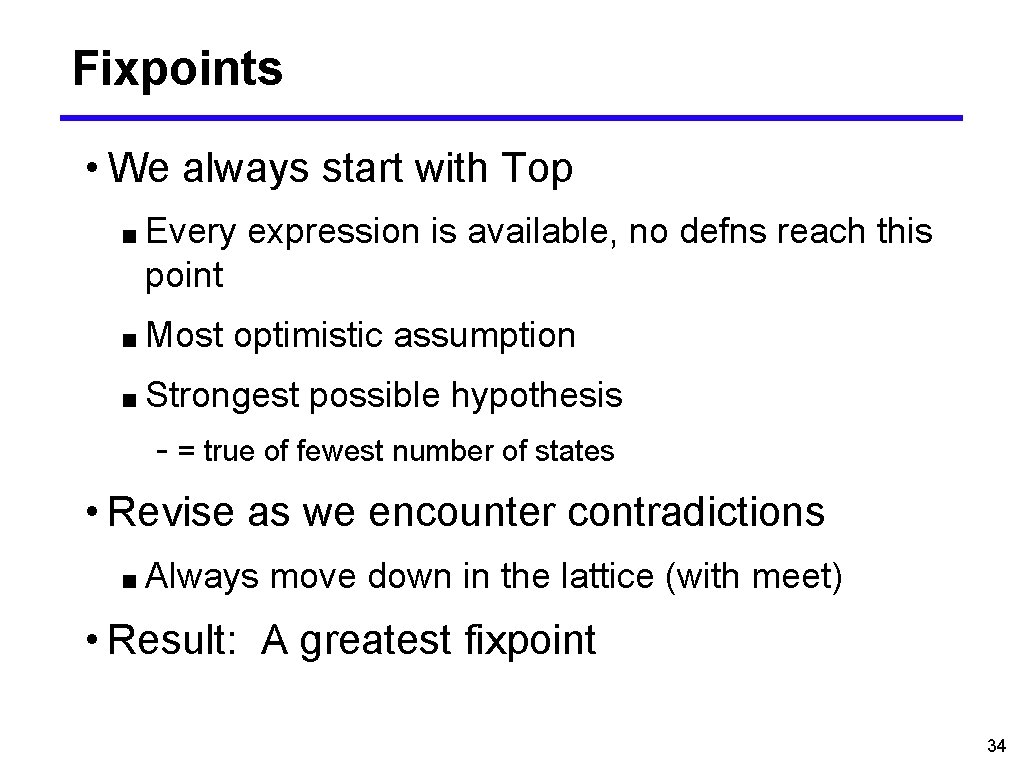
Fixpoints • We always start with Top ■ Every expression is available, no defns reach this point ■ Most optimistic assumption ■ Strongest possible hypothesis - = true of fewest number of states • Revise as we encounter contradictions ■ Always move down in the lattice (with meet) • Result: A greatest fixpoint 34

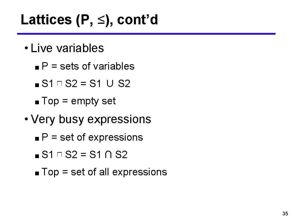
Lattices (P, ≤), cont’d • Live variables ■P = sets of variables ■ S 1 ⊓ S 2 = S 1 ∪ S 2 ■ Top = empty set • Very busy expressions ■P = set of expressions ■ S 1 ⊓ S 2 = S 1 ∩ S 2 ■ Top = set of all expressions 35

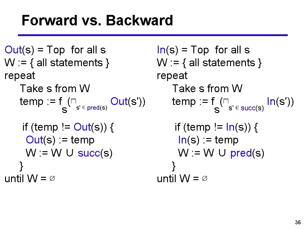
Forward vs. Backward Out(s) = Top for all s W : = { all statements } repeat Take s from W temp : = f (⊓s′ ∊ pred(s) Out(s′)) s In(s) = Top for all s W : = { all statements } repeat Take s from W temp : = f (⊓s′ ∊ succ(s) In(s′)) s if (temp != Out(s)) { Out(s) : = temp W : = W ∪ succ(s) } until W = ∅ if (temp != In(s)) { In(s) : = temp W : = W ∪ pred(s) } until W = ∅ 36

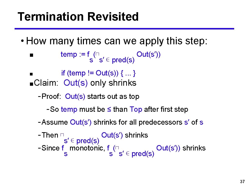
Termination Revisited • How many times can we apply this step: ■ temp : = f (⊓ Out(s′)) s s′ ∊ pred(s) ■ if (temp != Out(s)) {. . . } ■Claim: Out(s) only shrinks - Proof: Out(s) starts out as top - So temp must be ≤ than Top after first step - Assume Out(s′) shrinks for all predecessors s′ of s - Then ⊓ Out(s′) shrinks s′ ∊ pred(s) - Since f monotonic, f (⊓ Out(s′)) shrinks s s s′ ∊ pred(s) 37

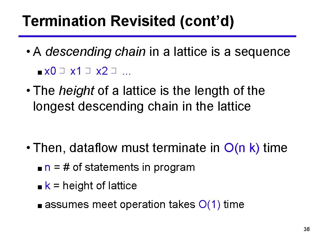
Termination Revisited (cont’d) • A descending chain in a lattice is a sequence ■ x 0 ⊐ x 1 ⊐ x 2 ⊐. . . • The height of a lattice is the length of the longest descending chain in the lattice • Then, dataflow must terminate in O(n k) time ■n = # of statements in program ■k = height of lattice ■ assumes meet operation takes O(1) time 38

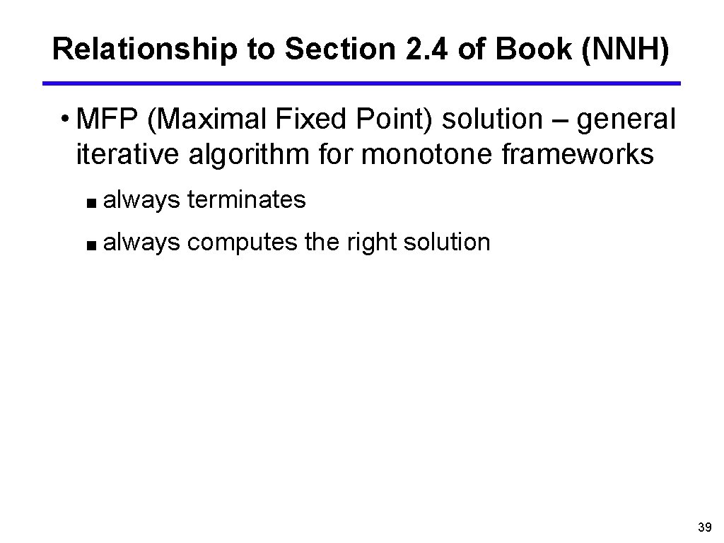
Relationship to Section 2. 4 of Book (NNH) • MFP (Maximal Fixed Point) solution – general iterative algorithm for monotone frameworks ■ always terminates ■ always computes the right solution 39

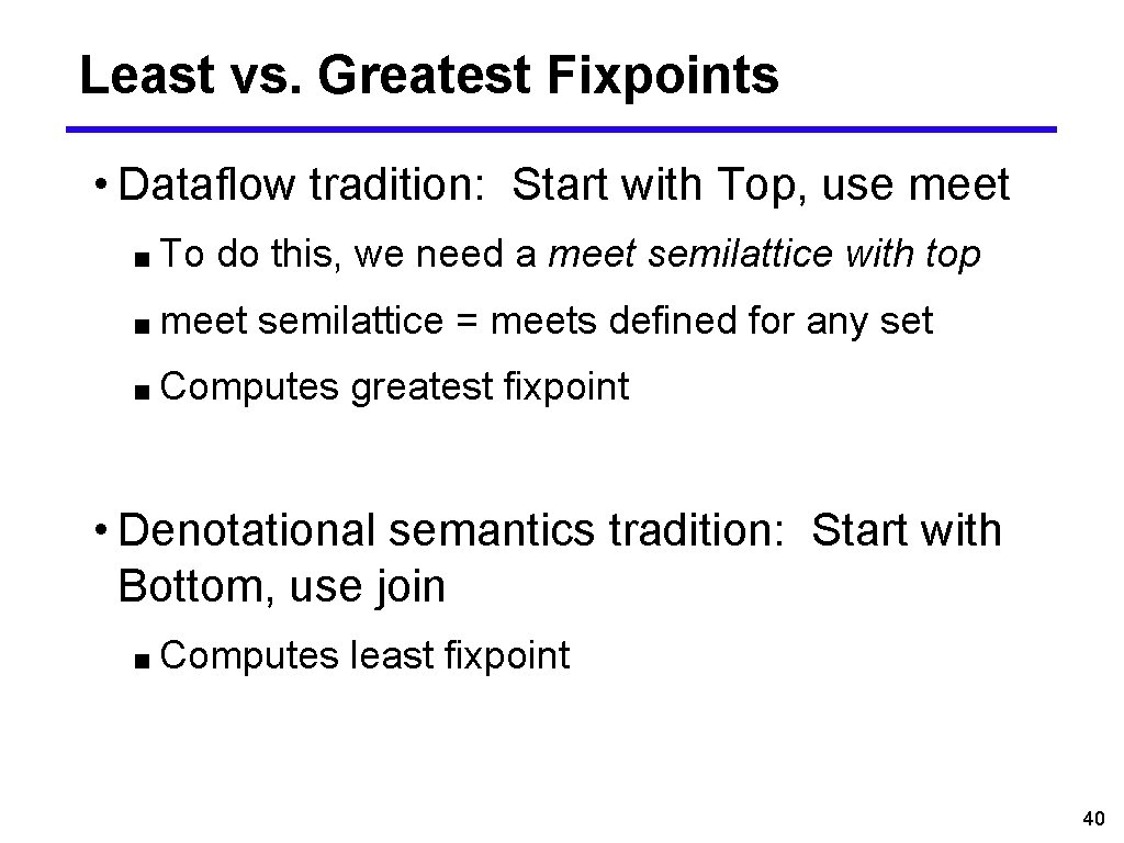
Least vs. Greatest Fixpoints • Dataflow tradition: Start with Top, use meet ■ To do this, we need a meet semilattice with top ■ meet semilattice = meets defined for any set ■ Computes greatest fixpoint • Denotational semantics tradition: Start with Bottom, use join ■ Computes least fixpoint 40

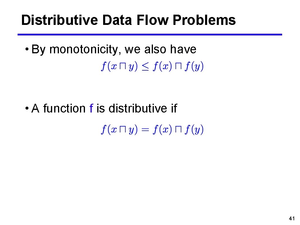
Distributive Data Flow Problems • By monotonicity, we also have • A function f is distributive if 41

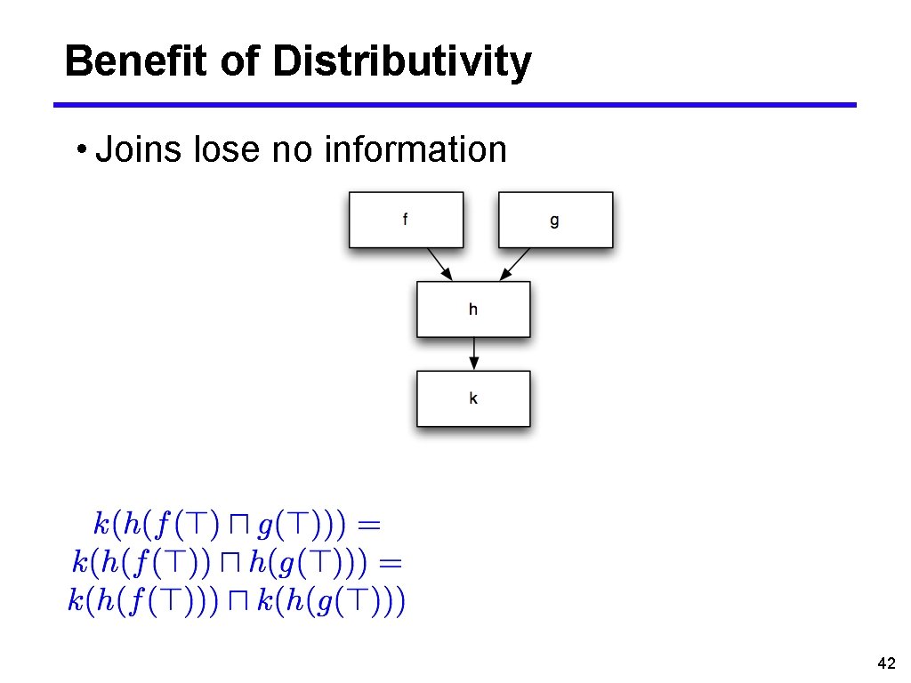
Benefit of Distributivity • Joins lose no information 42

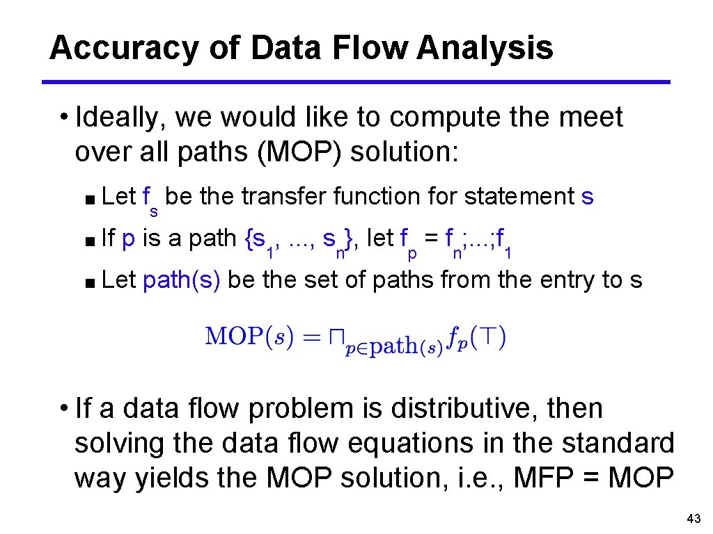
Accuracy of Data Flow Analysis • Ideally, we would like to compute the meet over all paths (MOP) solution: ■ Let ■ If fs be the transfer function for statement s p is a path {s 1, . . . , sn}, let fp = fn; . . . ; f 1 ■ Let path(s) be the set of paths from the entry to s • If a data flow problem is distributive, then solving the data flow equations in the standard way yields the MOP solution, i. e. , MFP = MOP 43

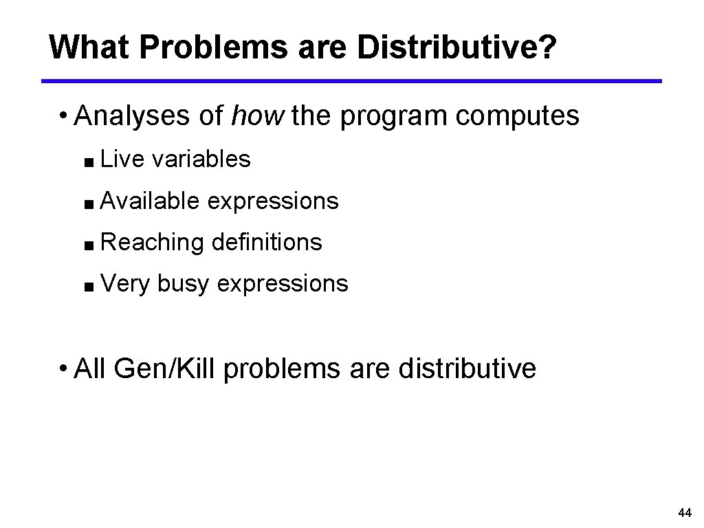
What Problems are Distributive? • Analyses of how the program computes ■ Live variables ■ Available expressions ■ Reaching definitions ■ Very busy expressions • All Gen/Kill problems are distributive 44

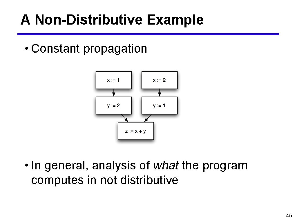
A Non-Distributive Example • Constant propagation • In general, analysis of what the program computes in not distributive 45

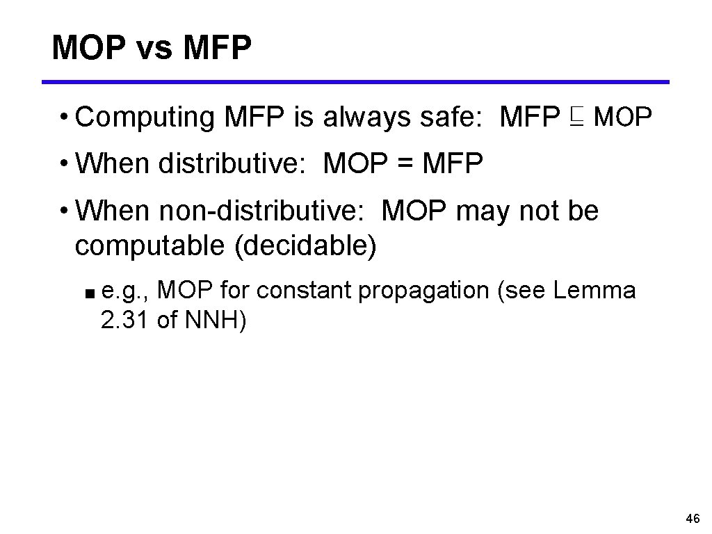
MOP vs MFP • Computing MFP is always safe: MFP ⊑ MOP • When distributive: MOP = MFP • When non-distributive: MOP may not be computable (decidable) ■ e. g. , MOP for constant propagation (see Lemma 2. 31 of NNH) 46

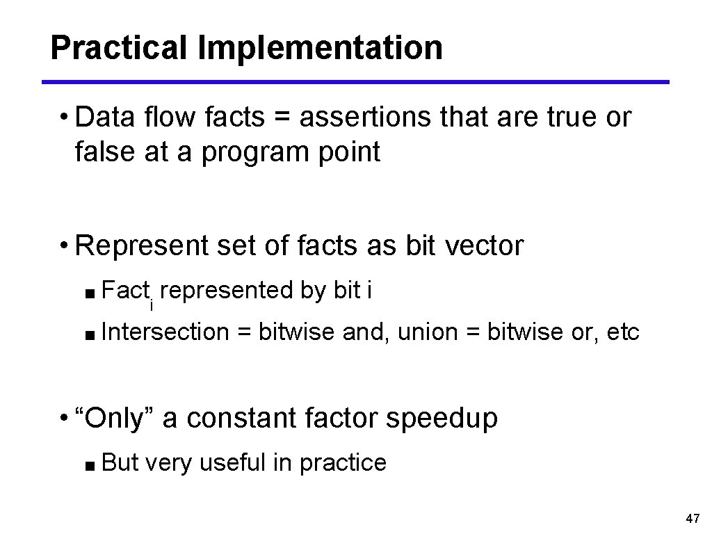
Practical Implementation • Data flow facts = assertions that are true or false at a program point • Represent set of facts as bit vector ■ Fact represented by bit i i ■ Intersection = bitwise and, union = bitwise or, etc • “Only” a constant factor speedup ■ But very useful in practice 47

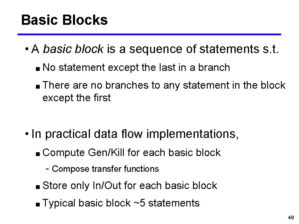
Basic Blocks • A basic block is a sequence of statements s. t. ■ No statement except the last in a branch ■ There are no branches to any statement in the block except the first • In practical data flow implementations, ■ Compute Gen/Kill for each basic block - Compose transfer functions ■ Store only In/Out for each basic block ■ Typical basic block ~5 statements 48

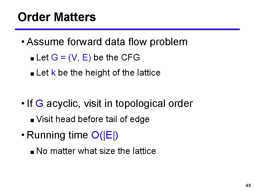
Order Matters • Assume forward data flow problem ■ Let G = (V, E) be the CFG ■ Let k be the height of the lattice • If G acyclic, visit in topological order ■ Visit head before tail of edge • Running time O(|E|) ■ No matter what size the lattice 49

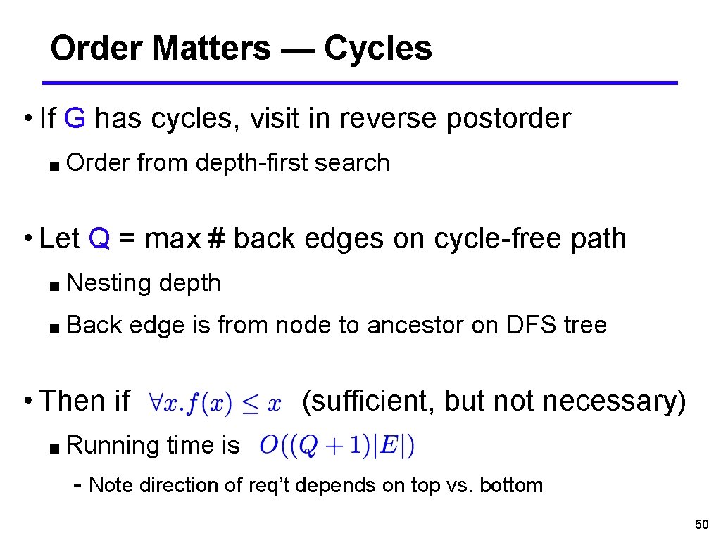
Order Matters — Cycles • If G has cycles, visit in reverse postorder ■ Order from depth-first search • Let Q = max # back edges on cycle-free path ■ Nesting ■ Back depth edge is from node to ancestor on DFS tree • Then if ■ Running (sufficient, but not necessary) time is - Note direction of req’t depends on top vs. bottom 50

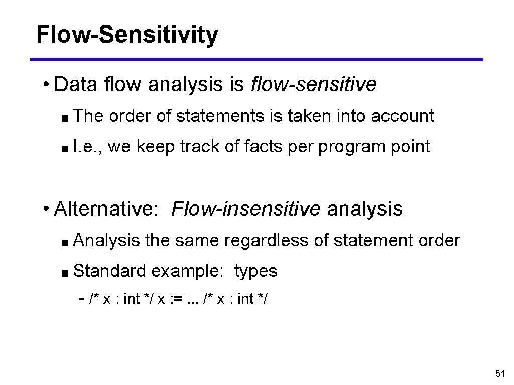
Flow-Sensitivity • Data flow analysis is flow-sensitive ■ The order of statements is taken into account ■ I. e. , we keep track of facts per program point • Alternative: Flow-insensitive analysis ■ Analysis the same regardless of statement order ■ Standard example: types - /* x : int */ x : =. . . /* x : int */ 51

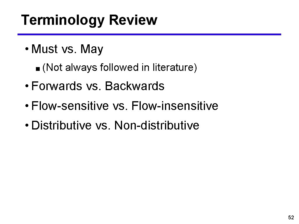
Terminology Review • Must vs. May ■ (Not always followed in literature) • Forwards vs. Backwards • Flow-sensitive vs. Flow-insensitive • Distributive vs. Non-distributive 52

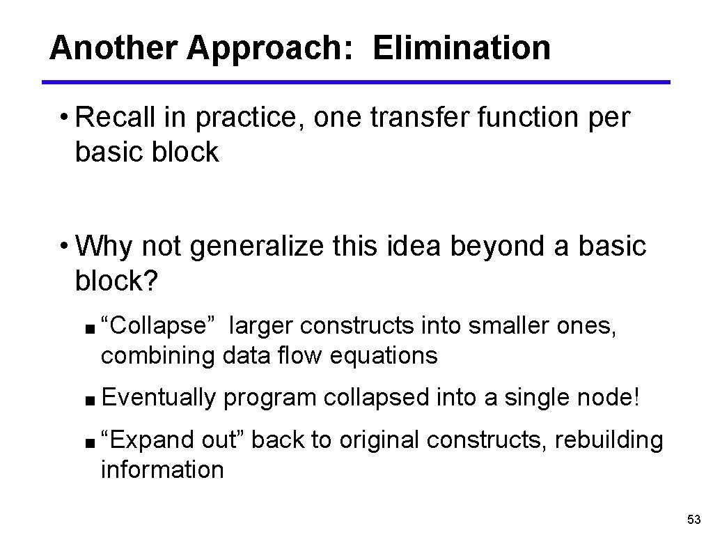
Another Approach: Elimination • Recall in practice, one transfer function per basic block • Why not generalize this idea beyond a basic block? ■ “Collapse” larger constructs into smaller ones, combining data flow equations ■ Eventually program collapsed into a single node! ■ “Expand out” back to original constructs, rebuilding information 53

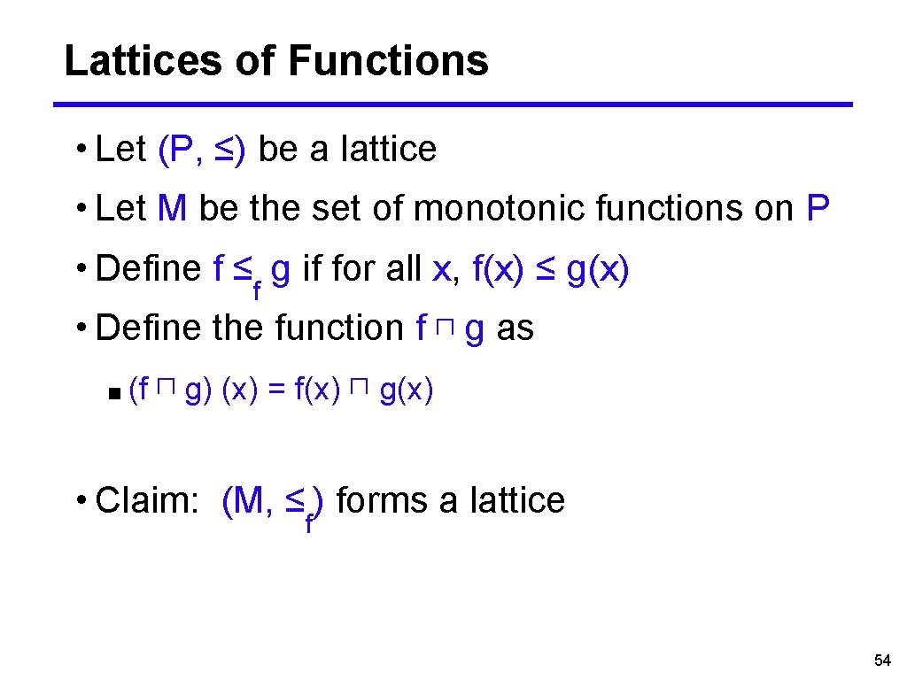
Lattices of Functions • Let (P, ≤) be a lattice • Let M be the set of monotonic functions on P • Define f ≤ g if for all x, f(x) ≤ g(x) f • Define the function f ⊓ g as ■ (f ⊓ g) (x) = f(x) ⊓ g(x) • Claim: (M, ≤ ) forms a lattice f 54

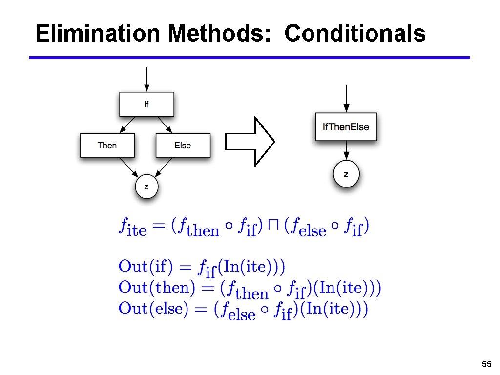
Elimination Methods: Conditionals 55

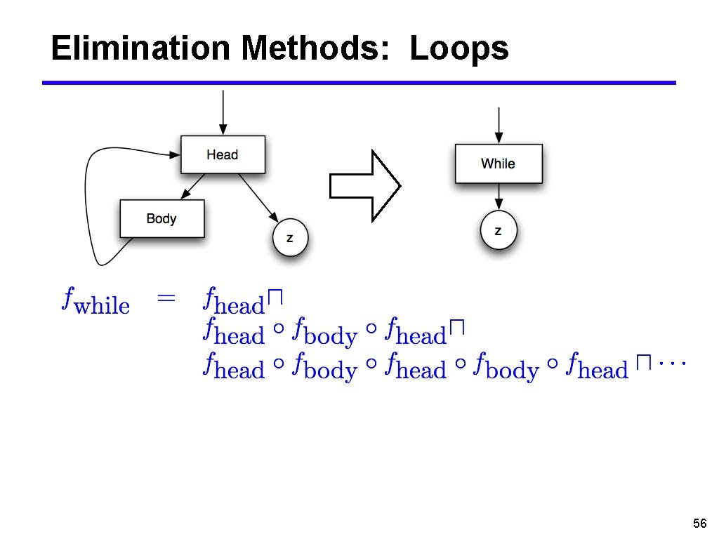
Elimination Methods: Loops 56

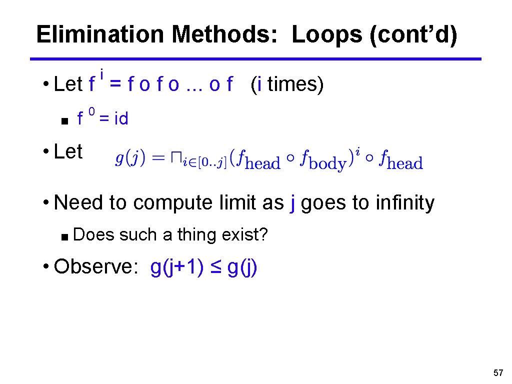
Elimination Methods: Loops (cont’d) i • Let f = f o. . . o f (i times) ■ 0 f = id • Let • Need to compute limit as j goes to infinity ■ Does such a thing exist? • Observe: g(j+1) ≤ g(j) 57

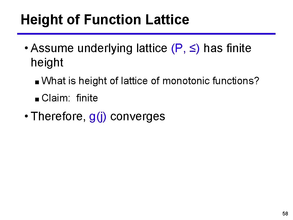
Height of Function Lattice • Assume underlying lattice (P, ≤) has finite height ■ What is height of lattice of monotonic functions? ■ Claim: finite • Therefore, g(j) converges 58

Non-Reducible Flow Graphs • Elimination methods usually only applied to reducible flow graphs ■ Ones that can be collapsed ■ Standard constructs yield only reducible flow graphs • Unrestricted goto can yield non-reducible graphs 59

Comments • Can also do backwards elimination ■ Not quite as nice (regions are usually single entry but often not single exit) • For bit-vector problems, elimination efficient ■ Easy to compose functions, compute meet, etc. • Elimination originally seemed like it might be faster than iteration ■ Not really the case 60

Data Flow Analysis and Functions • What happens at a function call? ■ Lots of proposed solutions in data flow analysis literature • In practice, only analyze one procedure at a time • Consequences ■ Call to function kills all data flow facts ■ May be able to improve depending on language, e. g. , function call may not affect locals 61

More Terminology • An analysis that models only a single function at a time is intraprocedural • An analysis that takes multiple functions into account is interprocedural • An analysis that takes the whole program into account is. . . guess? • Note: global analysis means “more than one basic block, ” but still within a function 62

Data Flow Analysis and The Heap • Data Flow is good at analyzing local variables ■ But what about values stored in the heap? ■ Not modeled in traditional data flow • In practice: *x : = e ■ Assume all data flow facts killed (!) ■ Or, assume write through x may affect any variable whose address has been taken • In general, hard to analyze pointers 63

Data Flow Analysis and Optimization • Moore’s Law: Hardware advances double computing power every 18 months. • Proebsting’s Law: Compiler advances double computing power every 18 years. 64