CS 412 Intro to Data Mining Chapter 2

CS 412 Intro. to Data Mining Chapter 2. Getting to Know Your Data Jiawei Han, Computer Science, Univ. Illinois at Urbana-Champaign, 2017 1

February 10, 2022 Data Mining: Concepts and Techniques 2

Chapter 2. Getting to Know Your Data 3 q Data Objects and Attribute Types q Basic Statistical Descriptions of Data q Data Visualization q Measuring Data Similarity and Dissimilarity q Summary

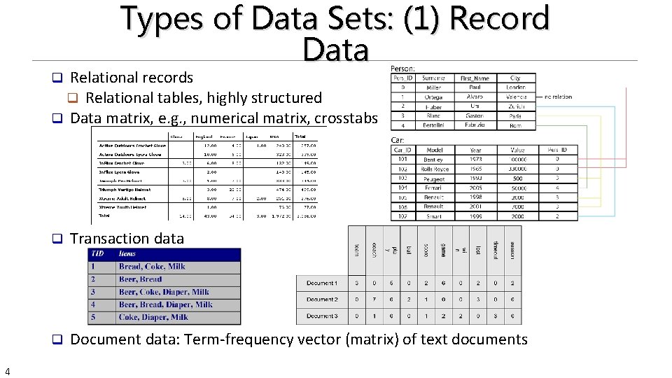
Types of Data Sets: (1) Record Data Relational records q Relational tables, highly structured q Data matrix, e. g. , numerical matrix, crosstabs q 4 q Transaction data q Document data: Term-frequency vector (matrix) of text documents

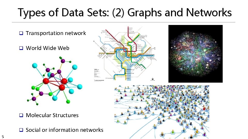
Types of Data Sets: (2) Graphs and Networks 5 q Transportation network q World Wide Web q Molecular Structures q Social or information networks

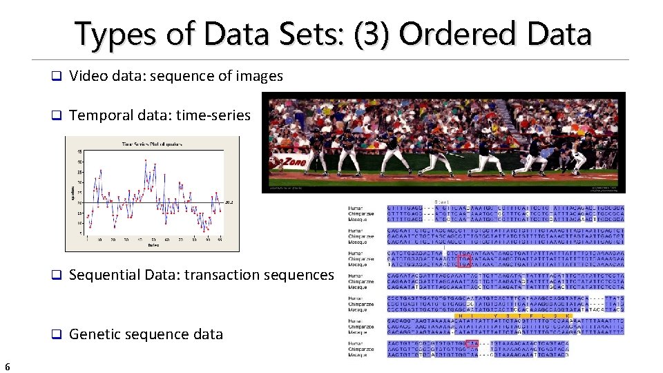
Types of Data Sets: (3) Ordered Data 6 q Video data: sequence of images q Temporal data: time-series q Sequential Data: transaction sequences q Genetic sequence data

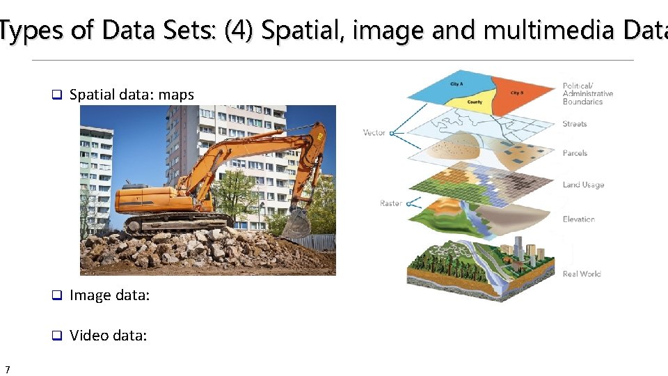
Types of Data Sets: (4) Spatial, image and multimedia Data 7 q Spatial data: maps q Image data: q Video data:

Important Characteristics of Structured Data q Dimensionality q Curse of dimensionality q Sparsity q Only presence counts q Resolution q Patterns depend on the scale q Distribution q Centrality and dispersion 8

Data Objects 9 q Data sets are made up of data objects q A data object represents an entity q Examples: q sales database: customers, store items, sales q medical database: patients, treatments q university database: students, professors, courses q Also called samples , examples, instances, data points, objects, tuples q Data objects are described by attributes q Database rows → data objects; columns → attributes

Attributes Attribute (or dimensions, features, variables) q A data field, representing a characteristic or feature of a data object. q E. g. , customer _ID, name, address q Types: q Nominal (e. g. , red, blue) q Binary (e. g. , {true, false}) q Ordinal (e. g. , {freshman, sophomore, junior, senior}) q Numeric: quantitative q Interval-scaled: 100○C is interval scales q Ratio-scaled: 100○K is ratio scaled since it is twice as high as 50 ○K q Q 1: Is student ID a nominal, ordinal, or interval-scaled data? q Q 2: What about eye color? Or color in the color spectrum of physics? q 10

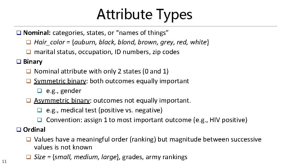
Attribute Types q Nominal: categories, states, or “names of things” Hair_color = {auburn, black, blond, brown, grey, red, white} q marital status, occupation, ID numbers, zip codes q Binary q Nominal attribute with only 2 states (0 and 1) q Symmetric binary: both outcomes equally important q e. g. , gender q Asymmetric binary: outcomes not equally important. q e. g. , medical test (positive vs. negative) q Convention: assign 1 to most important outcome (e. g. , HIV positive) q Ordinal q Values have a meaningful order (ranking) but magnitude between successive values is not known q Size = {small, medium, large}, grades, army rankings q 11

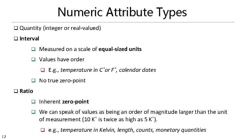
Numeric Attribute Types q Quantity (integer or real-valued) q Interval q Measured on a scale of equal-sized units q Values have order q q E. g. , temperature in C˚or F˚, calendar dates No true zero-point q Ratio q Inherent zero-point q We can speak of values as being an order of magnitude larger than the unit of measurement (10 K˚ is twice as high as 5 K˚). q 12 e. g. , temperature in Kelvin, length, counts, monetary quantities

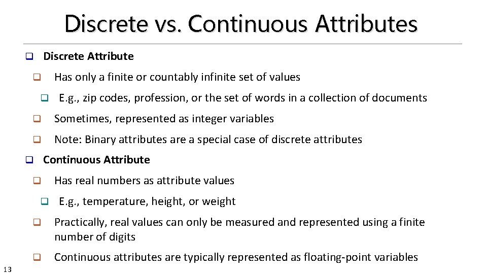
Discrete vs. Continuous Attributes Discrete Attribute q Has only a finite or countably infinite set of values q q q Sometimes, represented as integer variables q Note: Binary attributes are a special case of discrete attributes Continuous Attribute q q q 13 E. g. , zip codes, profession, or the set of words in a collection of documents Has real numbers as attribute values E. g. , temperature, height, or weight q Practically, real values can only be measured and represented using a finite number of digits q Continuous attributes are typically represented as floating-point variables

Chapter 2. Getting to Know Your Data 14 q Data Objects and Attribute Types q Basic Statistical Descriptions of Data q Data Visualization q Measuring Data Similarity and Dissimilarity q Summary

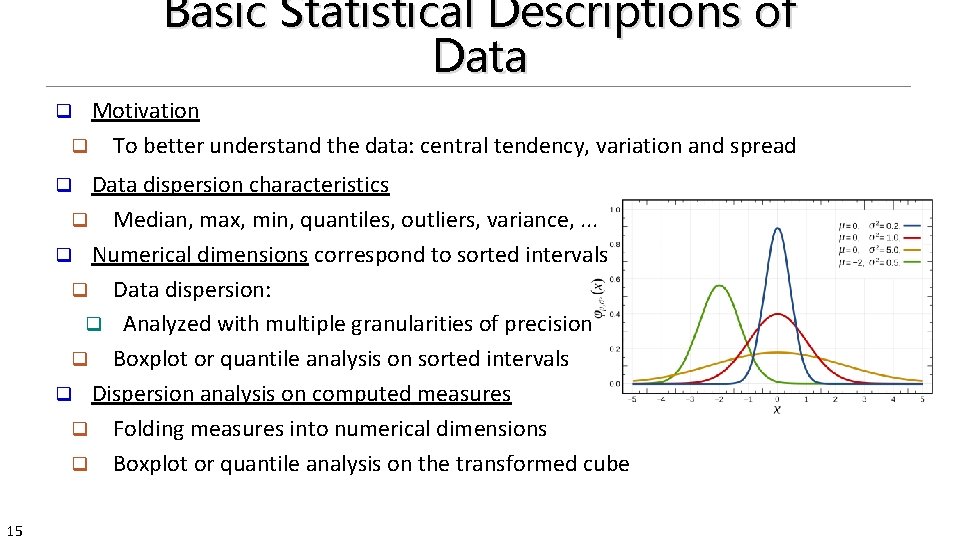
Basic Statistical Descriptions of Data Motivation q To better understand the data: central tendency, variation and spread q Data dispersion characteristics q Median, max, min, quantiles, outliers, variance, . . . q Numerical dimensions correspond to sorted intervals q Data dispersion: q Analyzed with multiple granularities of precision q Boxplot or quantile analysis on sorted intervals q Dispersion analysis on computed measures q Folding measures into numerical dimensions q Boxplot or quantile analysis on the transformed cube q 15

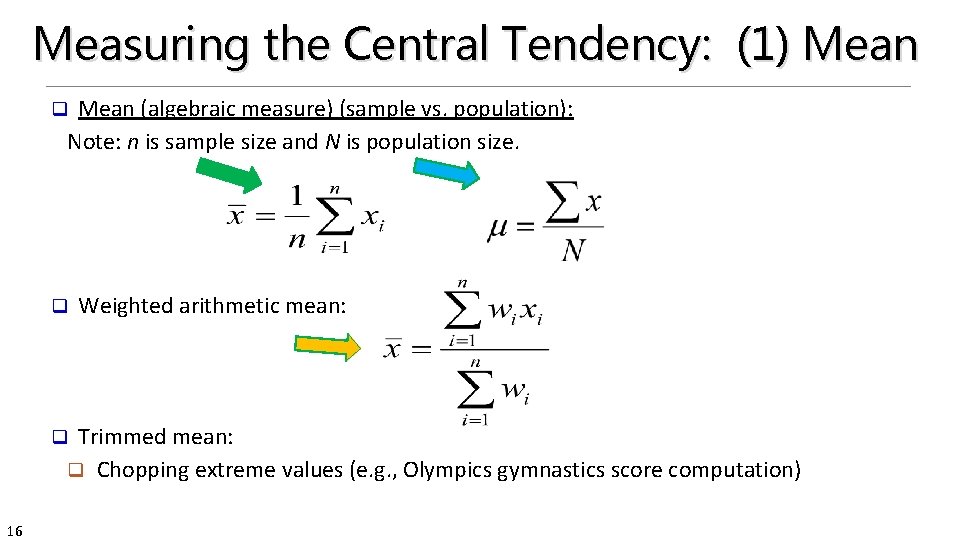
Measuring the Central Tendency: (1) Mean (algebraic measure) (sample vs. population): Note: n is sample size and N is population size. q q Weighted arithmetic mean: Trimmed mean: q Chopping extreme values (e. g. , Olympics gymnastics score computation) q 16

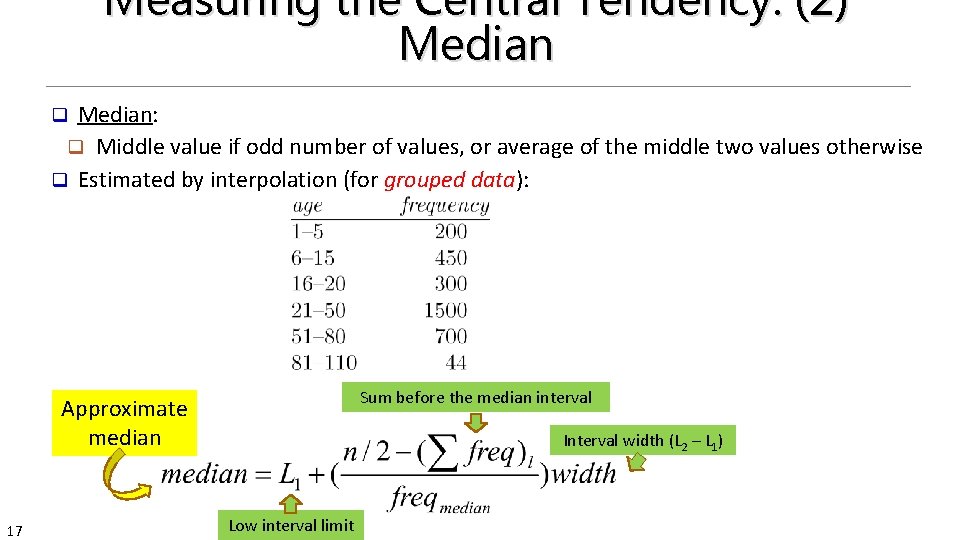
Measuring the Central Tendency: (2) Median: q Middle value if odd number of values, or average of the middle two values otherwise q Estimated by interpolation (for grouped data): q Sum before the median interval Approximate median 17 Interval width (L 2 – L 1) Low interval limit

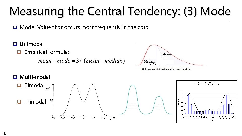
Measuring the Central Tendency: (3) Mode q Mode: Value that occurs most frequently in the data Unimodal q Empirical formula: q Multi-modal q Bimodal q q 18 Trimodal

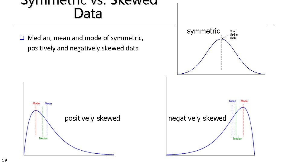
Symmetric vs. Skewed Data q Median, mean and mode of symmetric, positively and negatively skewed data positively skewed 19 symmetric negatively skewed

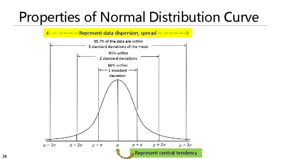
Properties of Normal Distribution Curve ← — ————Represent data dispersion, spread — ————→ 20 Represent central tendency

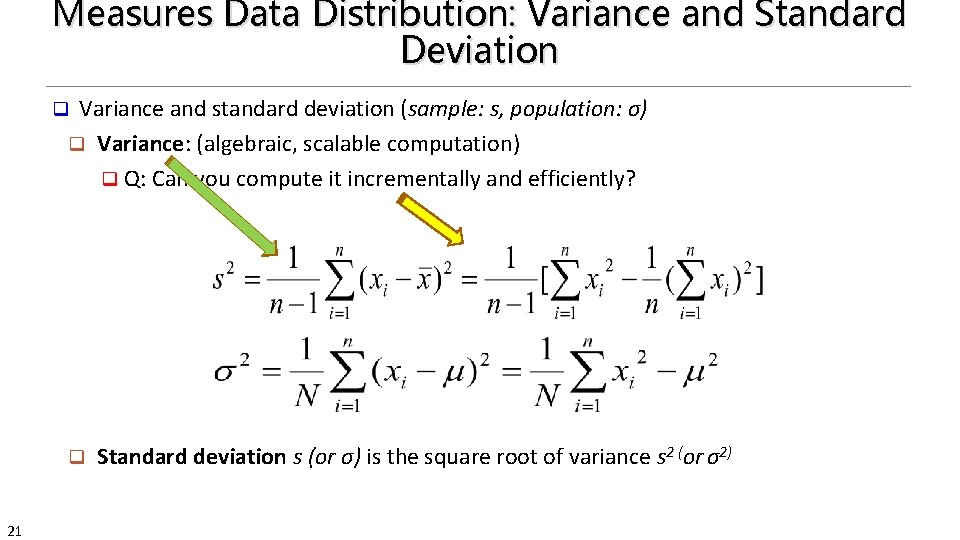
Measures Data Distribution: Variance and Standard Deviation Variance and standard deviation (sample: s, population: σ) q Variance: (algebraic, scalable computation) q Q: Can you compute it incrementally and efficiently? q q 21 Standard deviation s (or σ) is the square root of variance s 2 (or σ2)

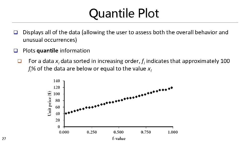
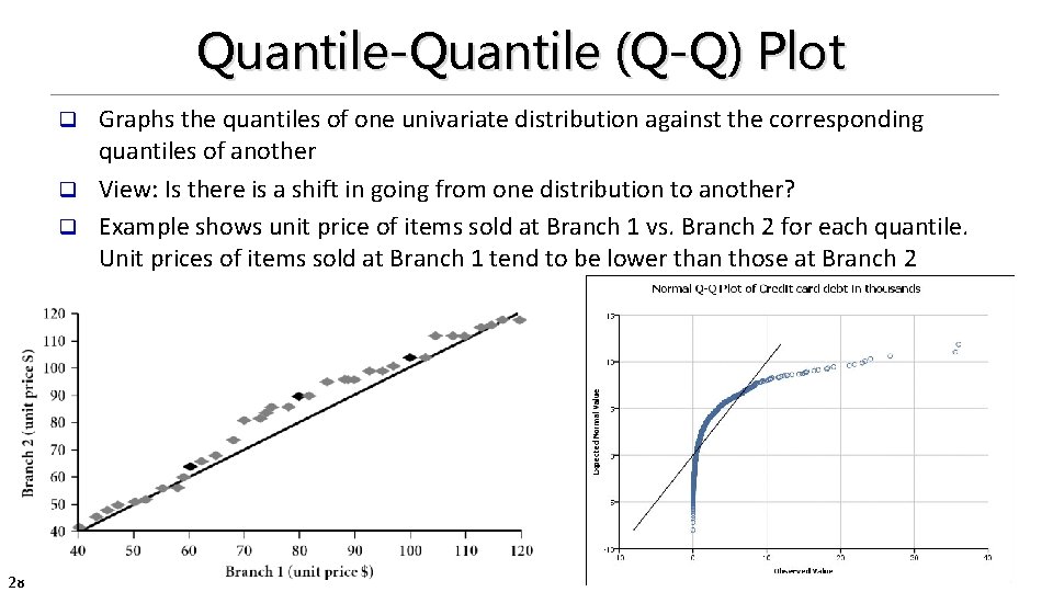
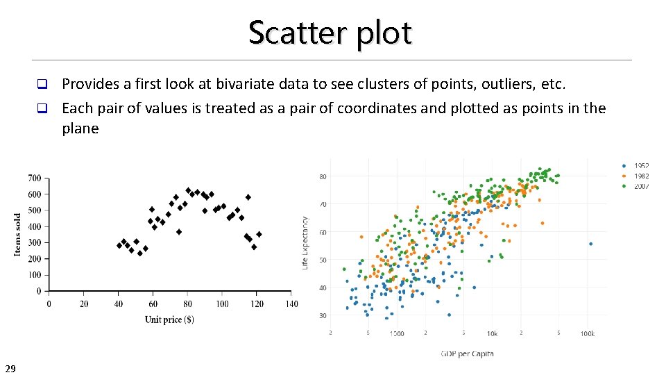
Graphic Displays of Basic Statistical Descriptions 22 q Boxplot: graphic display of five-number summary q Histogram: x-axis are values, y-axis repres. frequencies q Quantile plot: each value xi is paired with fi indicating that approximately 100 fi % of data are xi q Quantile-quantile (q-q) plot: graphs the quantiles of one univariant distribution against the corresponding quantiles of another q Scatter plot: each pair of values is a pair of coordinates and plotted as points in the plane

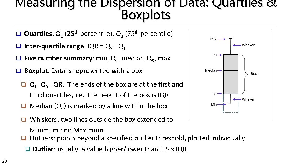
Measuring the Dispersion of Data: Quartiles & Boxplots q Quartiles: Q 1 (25 th percentile), Q 3 (75 th percentile) q Inter-quartile range: IQR = Q 3 – Q 1 q Five number summary: min, Q 1, median, Q 3, max q Boxplot: Data is represented with a box q Q 1, Q 3, IQR: The ends of the box are at the first and third quartiles, i. e. , the height of the box is IQR q Median (Q 2) is marked by a line within the box Whiskers: two lines outside the box extended to Minimum and Maximum q Outliers: points beyond a specified outlier threshold, plotted individually q q 23 Outlier: usually, a value higher/lower than 1. 5 x IQR

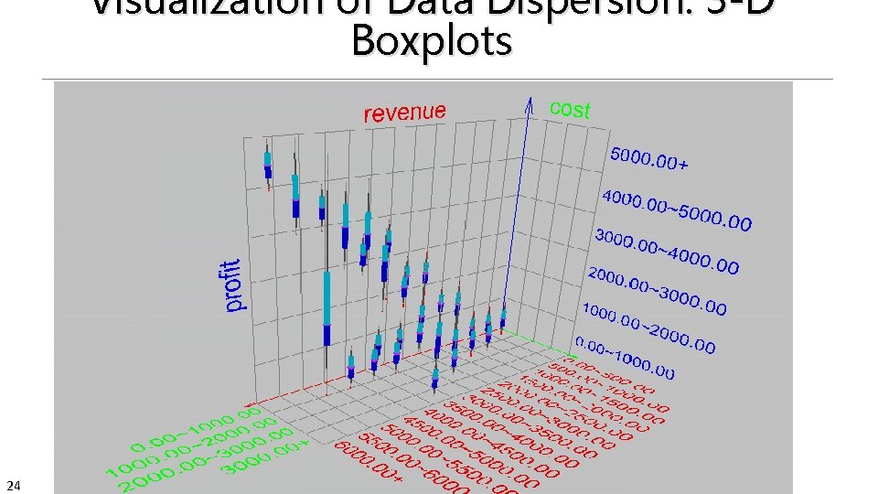
Visualization of Data Dispersion: 3 -D Boxplots 24

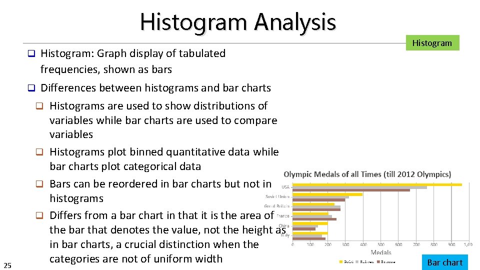
Histogram Analysis q Histogram: Graph display of tabulated frequencies, shown as bars Differences between histograms and bar charts q Histograms are used to show distributions of variables while bar charts are used to compare variables q Histograms plot binned quantitative data while bar charts plot categorical data q Bars can be reordered in bar charts but not in histograms q Differs from a bar chart in that it is the area of the bar that denotes the value, not the height as in bar charts, a crucial distinction when the categories are not of uniform width Histogram q 25 Bar chart

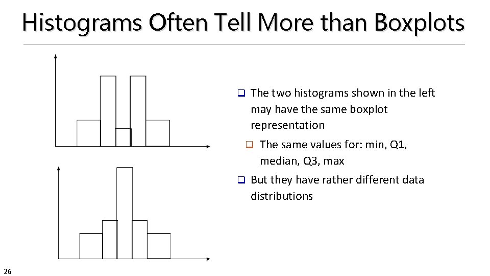
Histograms Often Tell More than Boxplots q The two histograms shown in the left may have the same boxplot representation q q 26 The same values for: min, Q 1, median, Q 3, max But they have rather different data distributions

Quantile Plot q Displays all of the data (allowing the user to assess both the overall behavior and unusual occurrences) q Plots quantile information q 27 For a data xi data sorted in increasing order, fi indicates that approximately 100 fi% of the data are below or equal to the value xi Data Mining: Concepts and Techniques

Quantile-Quantile (Q-Q) Plot Graphs the quantiles of one univariate distribution against the corresponding quantiles of another q View: Is there is a shift in going from one distribution to another? q Example shows unit price of items sold at Branch 1 vs. Branch 2 for each quantile. Unit prices of items sold at Branch 1 tend to be lower than those at Branch 2 q 28

Scatter plot Provides a first look at bivariate data to see clusters of points, outliers, etc. q Each pair of values is treated as a pair of coordinates and plotted as points in the plane q 29

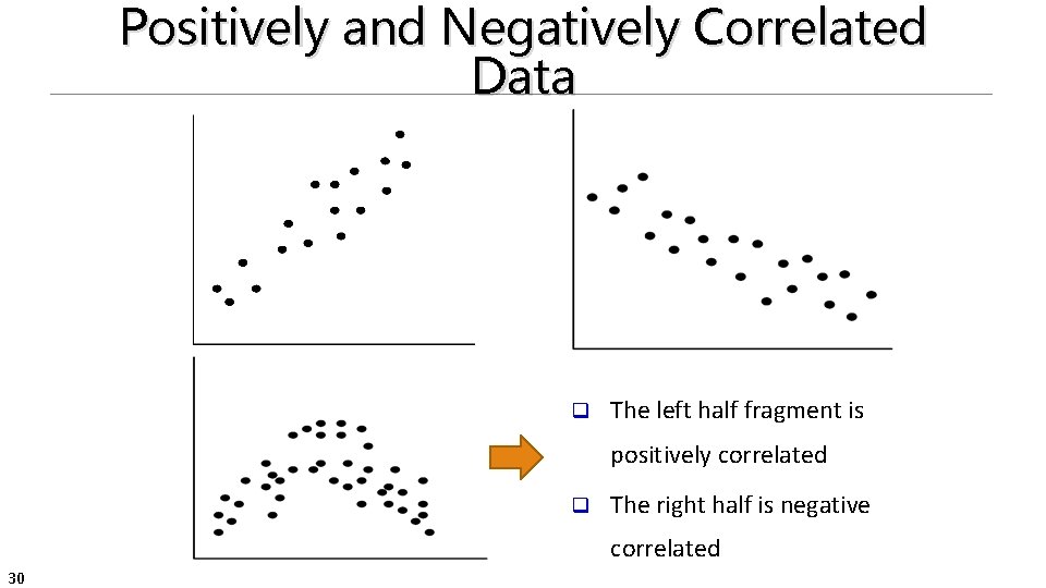
Positively and Negatively Correlated Data q The left half fragment is positively correlated q The right half is negative correlated 30

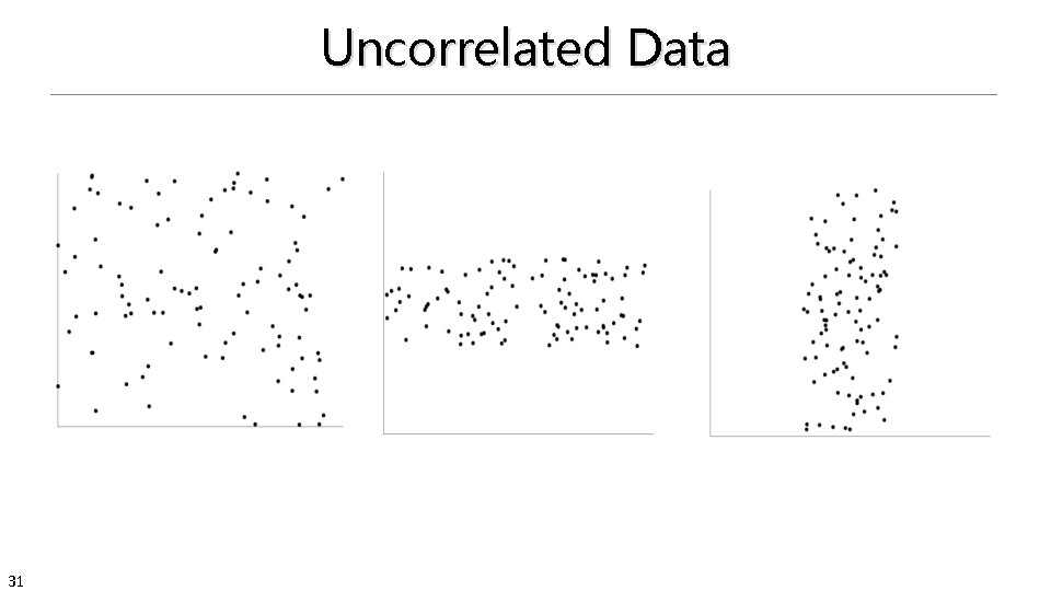
Uncorrelated Data 31

Chapter 2. Getting to Know Your Data 32 q Data Objects and Attribute Types q Basic Statistical Descriptions of Data q Data Visualization q Measuring Data Similarity and Dissimilarity q Summary

Data Visualization Why data visualization? q Gain insight into an information space by mapping data onto graphical primitives q Provide qualitative overview of large data sets q Search for patterns, trends, structure, irregularities, relationships among data q Help find interesting regions and suitable parameters for further quantitative analysis q Provide a visual proof of computer representations derived q Categorization of visualization methods: q Pixel-oriented visualization techniques q Geometric projection visualization techniques q Icon-based visualization techniques q Hierarchical visualization techniques q Visualizing complex data and relations q 33

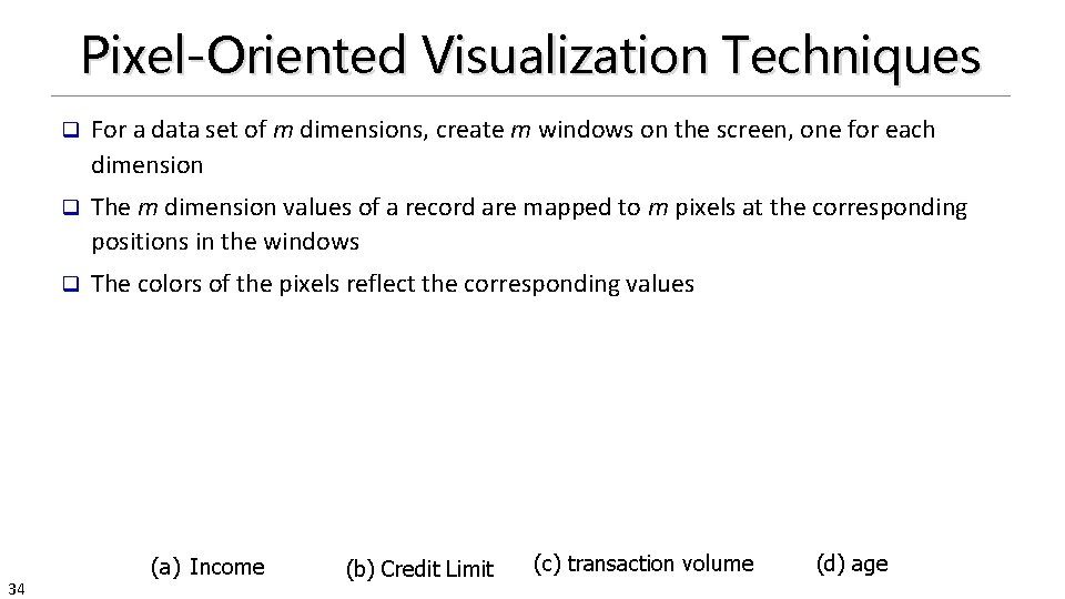
Pixel-Oriented Visualization Techniques 34 q For a data set of m dimensions, create m windows on the screen, one for each dimension q The m dimension values of a record are mapped to m pixels at the corresponding positions in the windows q The colors of the pixels reflect the corresponding values (a) Income (b) Credit Limit (c) transaction volume (d) age

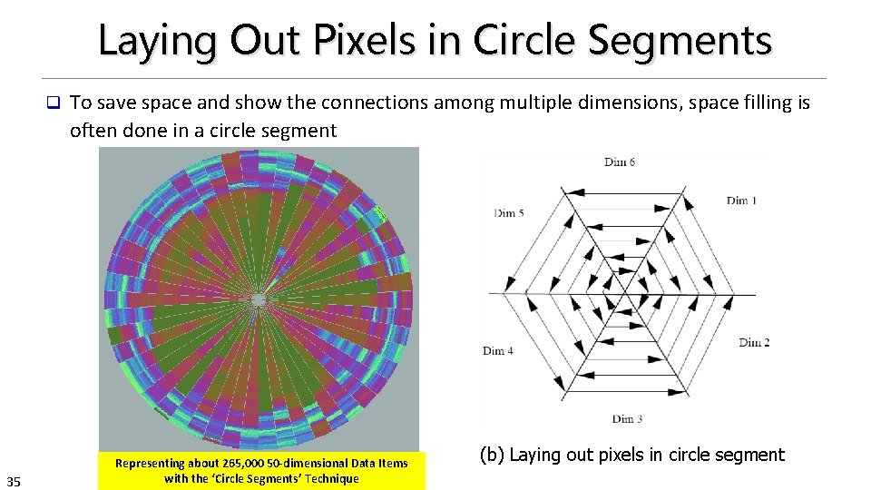
Laying Out Pixels in Circle Segments q To save space and show the connections among multiple dimensions, space filling is often done in a circle segment (a) Representing a data record in circle segment. Data Items Representing about 265, 000 50 -dimensional 35 with the ‘Circle Segments’ Technique (b) Laying out pixels in circle segment

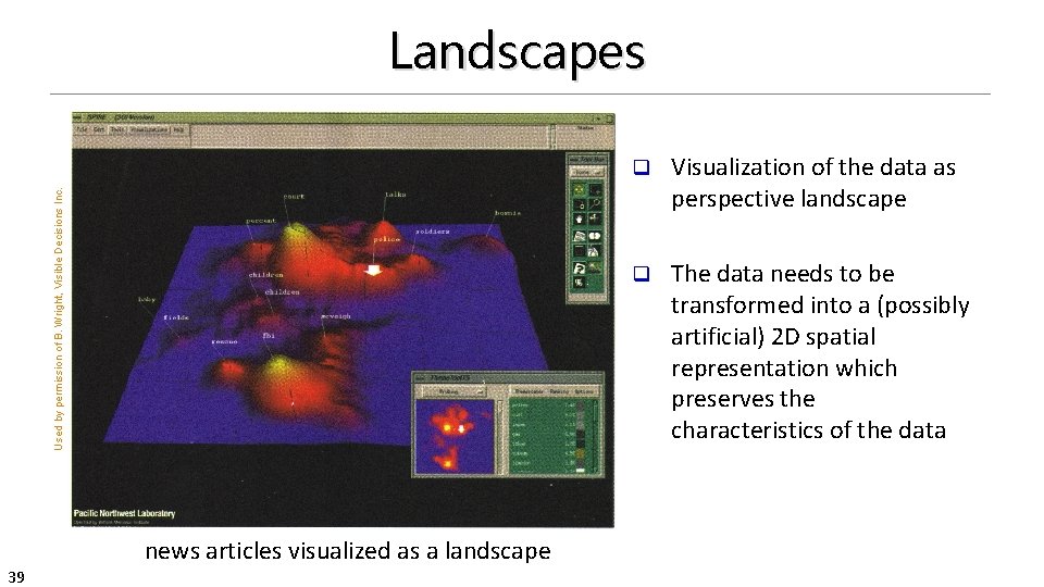
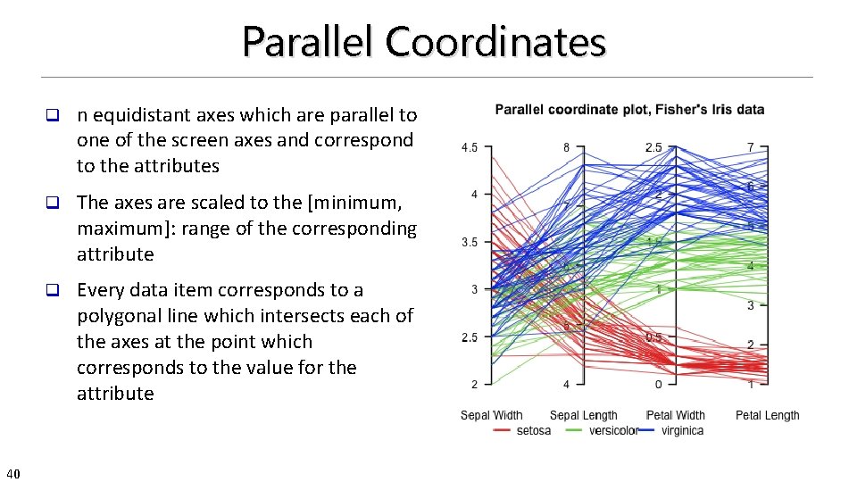
Geometric Projection Visualization Techniques 36 q Visualization of geometric transformations and projections of the data q Methods q Direct visualization q Scatterplot and scatterplot matrices q Landscapes q Projection pursuit technique: Help users find meaningful projections of multidimensional data q Prosection views q Hyperslice q Parallel coordinates

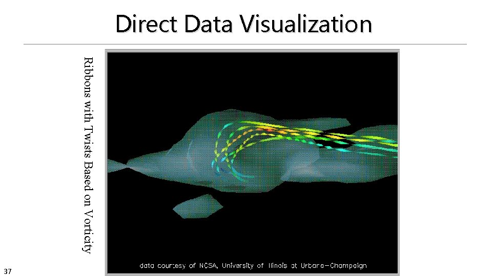
Direct Data Visualization Ribbons with Twists Based on Vorticity 37 Data Mining: Concepts and Techniques

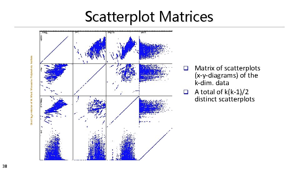
Used by ermission of M. Ward, Worcester Polytechnic Institute Scatterplot Matrices 38 Matrix of scatterplots (x-y-diagrams) of the k-dim. data q A total of k(k-1)/2 distinct scatterplots q

Used by permission of B. Wright, Visible Decisions Inc. Landscapes 39 news articles visualized as a landscape q Visualization of the data as perspective landscape q The data needs to be transformed into a (possibly artificial) 2 D spatial representation which preserves the characteristics of the data

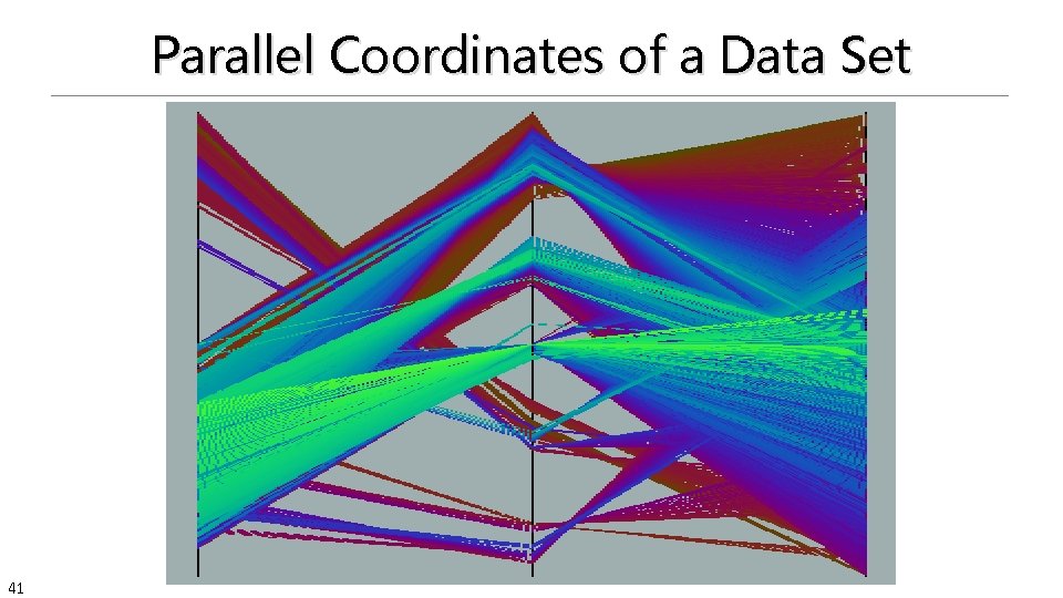
Parallel Coordinates 40 q n equidistant axes which are parallel to one of the screen axes and correspond to the attributes q The axes are scaled to the [minimum, maximum]: range of the corresponding attribute q Every data item corresponds to a polygonal line which intersects each of the axes at the point which corresponds to the value for the attribute

Parallel Coordinates of a Data Set 41

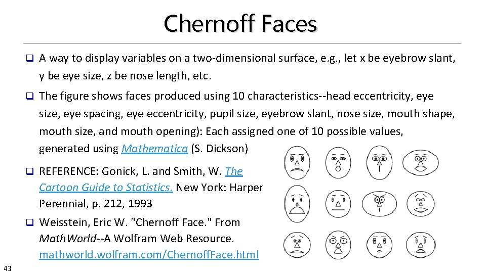
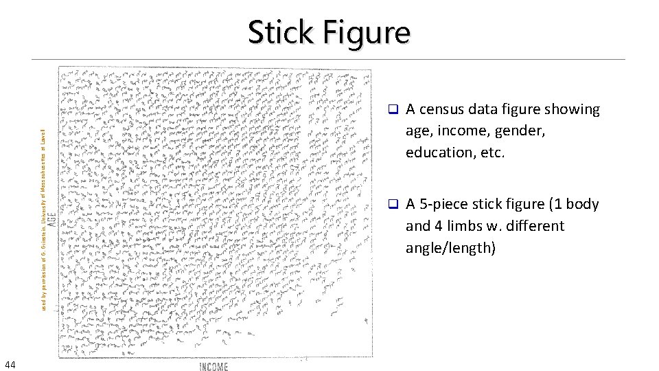
Icon-Based Visualization Techniques q Visualization of the data values as features of icons q Typical visualization methods q Chernoff Faces q Stick Figures q 42 General techniques q Shape coding: Use shape to represent certain information encoding q Color icons: Use color icons to encode more information q Tile bars: Use small icons to represent the relevant feature vectors in document retrieval

Chernoff Faces 43 q A way to display variables on a two-dimensional surface, e. g. , let x be eyebrow slant, y be eye size, z be nose length, etc. q The figure shows faces produced using 10 characteristics--head eccentricity, eye size, eye spacing, eye eccentricity, pupil size, eyebrow slant, nose size, mouth shape, mouth size, and mouth opening): Each assigned one of 10 possible values, generated using Mathematica (S. Dickson) q REFERENCE: Gonick, L. and Smith, W. The Cartoon Guide to Statistics. New York: Harper Perennial, p. 212, 1993 q Weisstein, Eric W. "Chernoff Face. " From Math. World--A Wolfram Web Resource. mathworld. wolfram. com/Chernoff. Face. html

used by permission of G. Grinstein, University of Massachusettes at Lowell Stick Figure 44 q A census data figure showing age, income, gender, education, etc. q A 5 -piece stick figure (1 body and 4 limbs w. different angle/length)

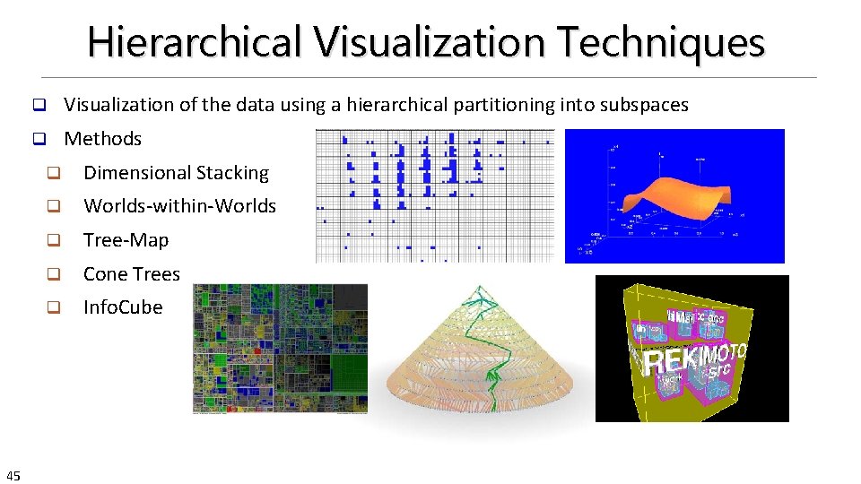
Hierarchical Visualization Techniques 45 q Visualization of the data using a hierarchical partitioning into subspaces q Methods q Dimensional Stacking q Worlds-within-Worlds q Tree-Map q Cone Trees q Info. Cube

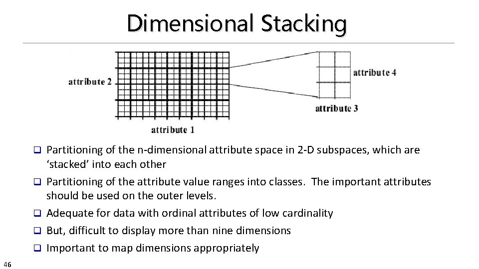
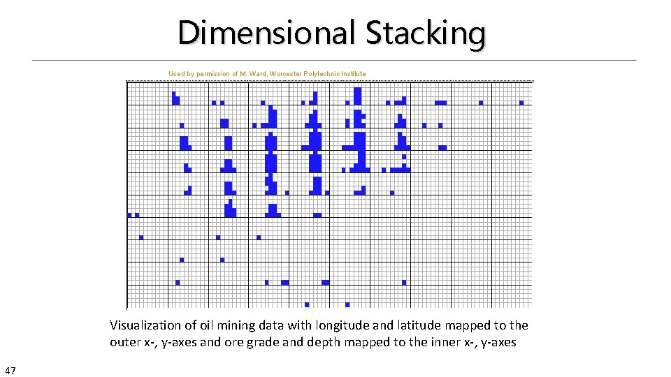
Dimensional Stacking q q q 46 Partitioning of the n-dimensional attribute space in 2 -D subspaces, which are ‘stacked’ into each other Partitioning of the attribute value ranges into classes. The important attributes should be used on the outer levels. Adequate for data with ordinal attributes of low cardinality But, difficult to display more than nine dimensions Important to map dimensions appropriately

Dimensional Stacking Used by permission of M. Ward, Worcester Polytechnic Institute Visualization of oil mining data with longitude and latitude mapped to the outer x-, y-axes and ore grade and depth mapped to the inner x-, y-axes 47

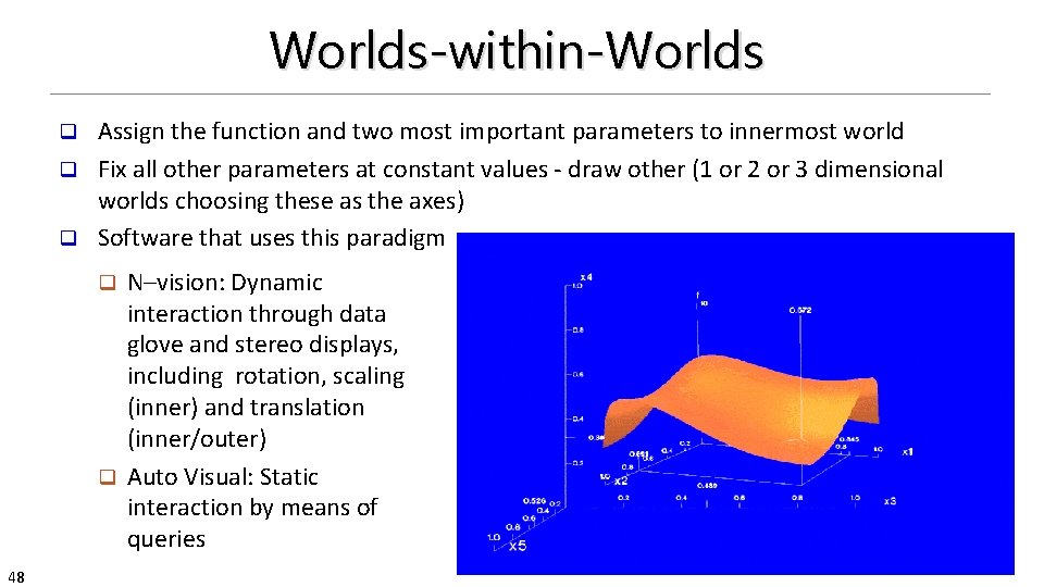
Worlds-within-Worlds Assign the function and two most important parameters to innermost world q Fix all other parameters at constant values - draw other (1 or 2 or 3 dimensional worlds choosing these as the axes) q Software that uses this paradigm q N–vision: Dynamic interaction through data glove and stereo displays, including rotation, scaling (inner) and translation (inner/outer) q Auto Visual: Static interaction by means of queries q 48

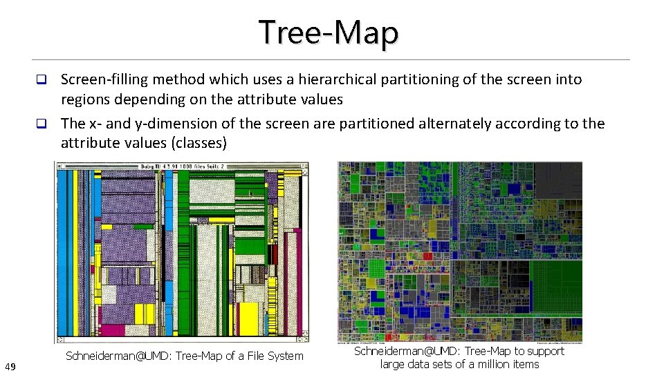
Tree-Map Screen-filling method which uses a hierarchical partitioning of the screen into regions depending on the attribute values q The x- and y-dimension of the screen are partitioned alternately according to the attribute values (classes) q 49 Schneiderman@UMD: Tree-Map of a File System Schneiderman@UMD: Tree-Map to support large data sets of a million items

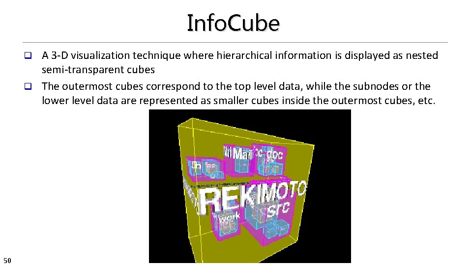
Info. Cube A 3 -D visualization technique where hierarchical information is displayed as nested semi-transparent cubes q The outermost cubes correspond to the top level data, while the subnodes or the lower level data are represented as smaller cubes inside the outermost cubes, etc. q 50

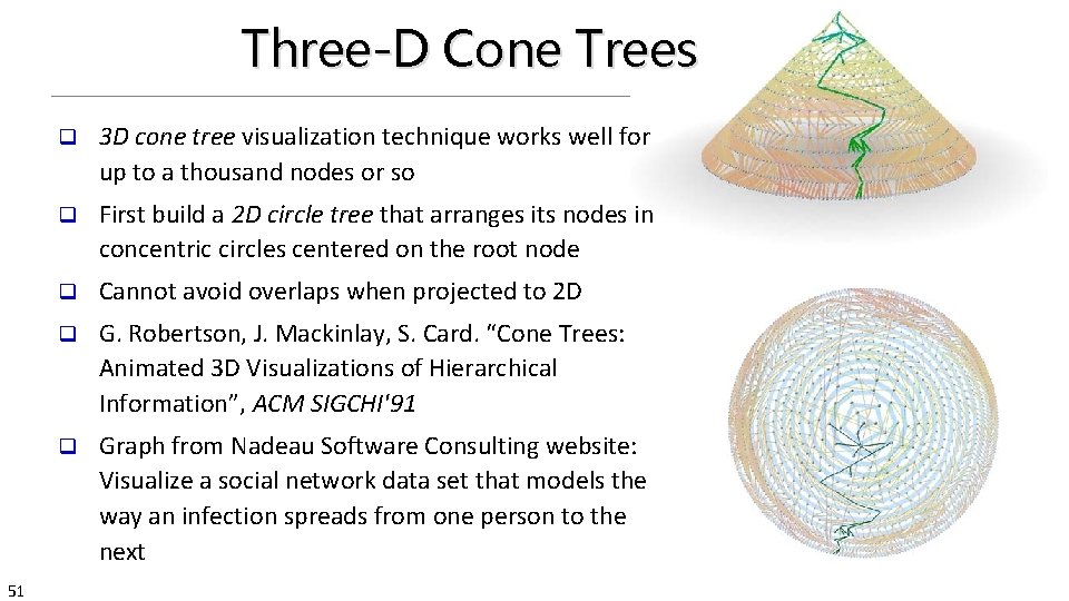
Three-D Cone Trees 51 q 3 D cone tree visualization technique works well for up to a thousand nodes or so q First build a 2 D circle tree that arranges its nodes in concentric circles centered on the root node q Cannot avoid overlaps when projected to 2 D q G. Robertson, J. Mackinlay, S. Card. “Cone Trees: Animated 3 D Visualizations of Hierarchical Information”, ACM SIGCHI'91 q Graph from Nadeau Software Consulting website: Visualize a social network data set that models the way an infection spreads from one person to the next

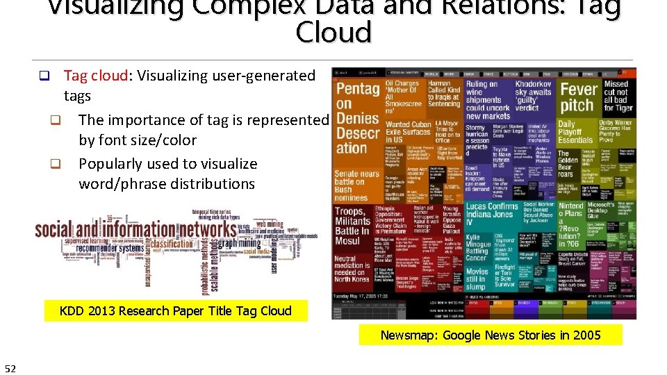
Visualizing Complex Data and Relations: Tag Cloud Tag cloud: Visualizing user-generated tags q The importance of tag is represented by font size/color q Popularly used to visualize word/phrase distributions q KDD 2013 Research Paper Title Tag Cloud Newsmap: Google News Stories in 2005 52

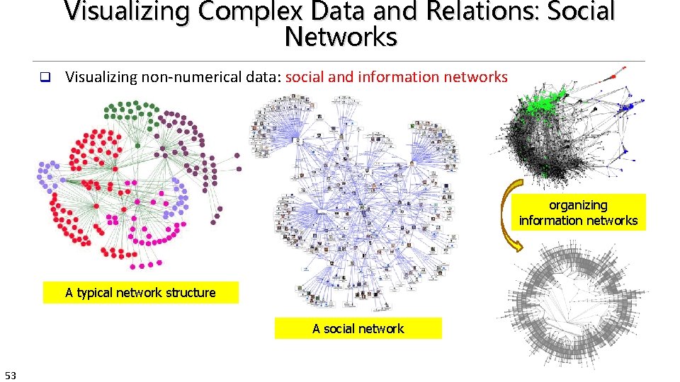
Visualizing Complex Data and Relations: Social Networks q Visualizing non-numerical data: social and information networks organizing information networks A typical network structure A social network 53

Chapter 2. Getting to Know Your Data 54 q Data Objects and Attribute Types q Basic Statistical Descriptions of Data q Data Visualization q Measuring Data Similarity and Dissimilarity q Summary

Similarity, Dissimilarity, and Proximity q q A real-valued function that quantifies the similarity between two objects q Measure how two data objects are alike: The higher value, the more alike q Often falls in the range [0, 1]: 0: no similarity; 1: completely similar q Dissimilarity (or distance) measure q Numerical measure of how different two data objects are q In some sense, the inverse of similarity: The lower, the more alike q Minimum dissimilarity is often 0 (i. e. , completely similar) q Range [0, 1] or [0, ∞) , depending on the definition q 55 Similarity measure or similarity function Proximity usually refers to either similarity or dissimilarity

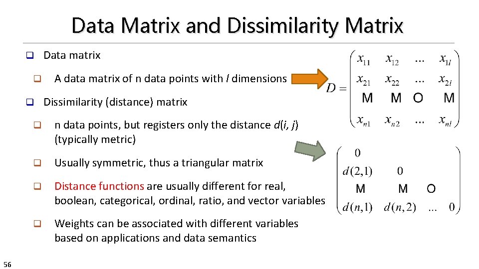
Data Matrix and Dissimilarity Matrix q q q 56 Data matrix A data matrix of n data points with l dimensions Dissimilarity (distance) matrix q n data points, but registers only the distance d(i, j) (typically metric) q Usually symmetric, thus a triangular matrix q Distance functions are usually different for real, boolean, categorical, ordinal, ratio, and vector variables q Weights can be associated with different variables based on applications and data semantics

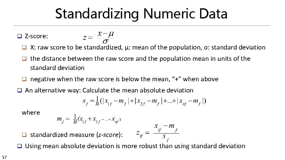
Standardizing Numeric Data q Z-score: q X: raw score to be standardized, μ: mean of the population, σ: standard deviation q the distance between the raw score and the population mean in units of the standard deviation q negative when the raw score is below the mean, “+” when above q An alternative way: Calculate the mean absolute deviation where q q 57 standardized measure (z-score): Using mean absolute deviation is more robust than using standard deviation

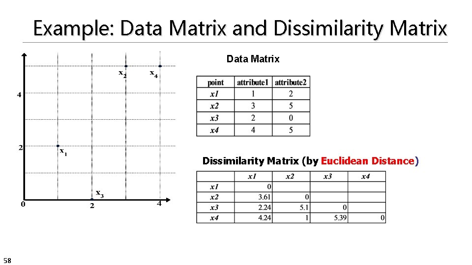
Example: Data Matrix and Dissimilarity Matrix Data Matrix Dissimilarity Matrix (by Euclidean Distance) 58

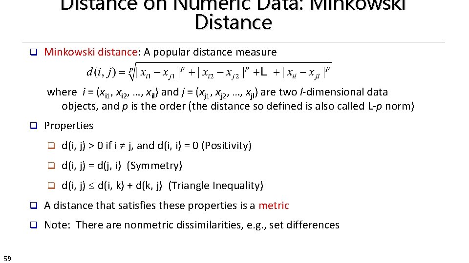
Distance on Numeric Data: Minkowski Distance q Minkowski distance: A popular distance measure where i = (xi 1, xi 2, …, xil) and j = (xj 1, xj 2, …, xjl) are two l-dimensional data objects, and p is the order (the distance so defined is also called L-p norm) q 59 Properties q d(i, j) > 0 if i ≠ j, and d(i, i) = 0 (Positivity) q d(i, j) = d(j, i) (Symmetry) q d(i, j) d(i, k) + d(k, j) (Triangle Inequality) q A distance that satisfies these properties is a metric q Note: There are nonmetric dissimilarities, e. g. , set differences

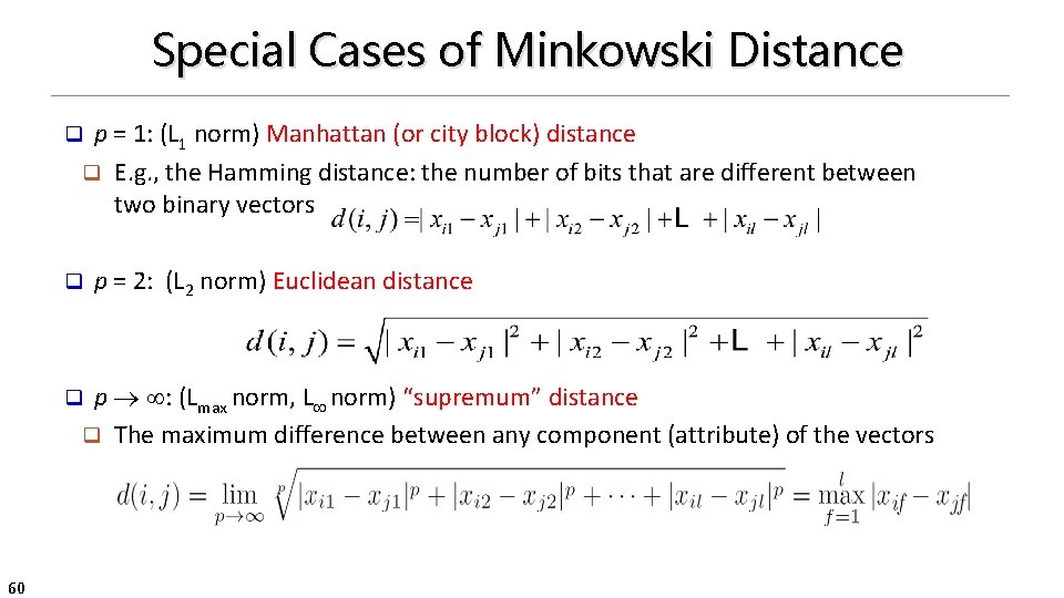
Special Cases of Minkowski Distance p = 1: (L 1 norm) Manhattan (or city block) distance q E. g. , the Hamming distance: the number of bits that are different between two binary vectors q q p = 2: (L 2 norm) Euclidean distance p : (Lmax norm, L norm) “supremum” distance q The maximum difference between any component (attribute) of the vectors q 60

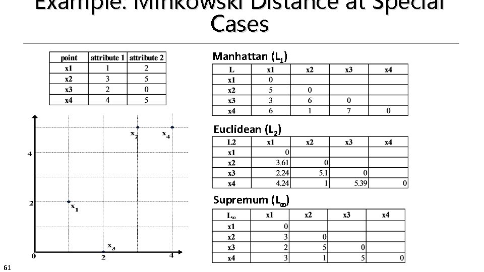
Example: Minkowski Distance at Special Cases Manhattan (L 1) Euclidean (L 2) Supremum (L ) 61

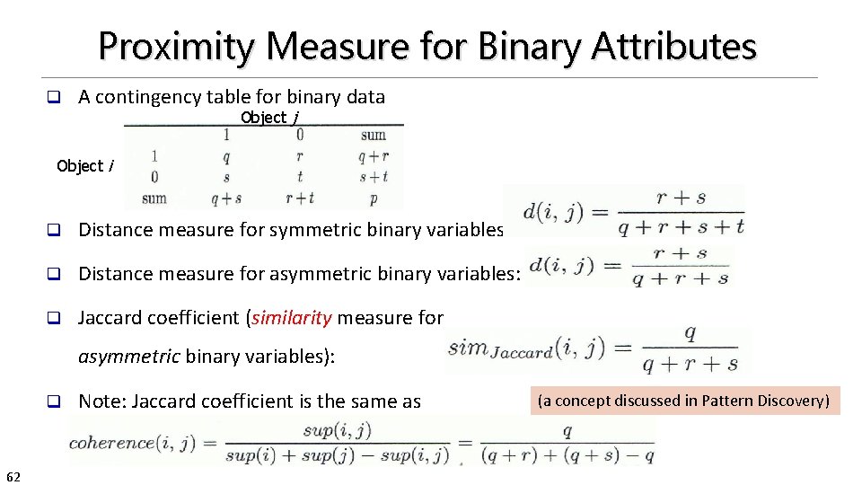
Proximity Measure for Binary Attributes q A contingency table for binary data Object j Object i q Distance measure for symmetric binary variables: q Distance measure for asymmetric binary variables: q Jaccard coefficient (similarity measure for asymmetric binary variables): q Note: Jaccard coefficient is the same as “coherence”: 62 (a concept discussed in Pattern Discovery)

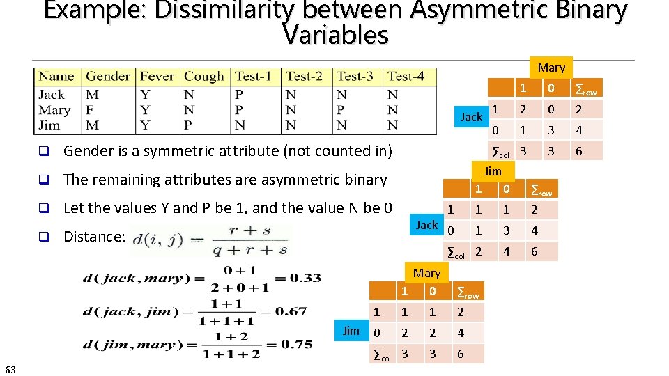
Example: Dissimilarity between Asymmetric Binary Variables Mary Jack q Gender is a symmetric attribute (not counted in) q The remaining attributes are asymmetric binary q Let the values Y and P be 1, and the value N be 0 q 63 1 0 ∑row 1 2 0 1 3 4 ∑col 3 3 6 Jim 1 0 ∑row 1 1 2 1 3 4 ∑col 2 4 6 1 Jack 0 Distance: Mary 1 0 ∑row 1 1 1 2 Jim 0 2 2 4 ∑col 3 3 6

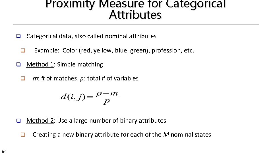
Proximity Measure for Categorical Attributes q q q 64 Categorical data, also called nominal attributes Example: Color (red, yellow, blue, green), profession, etc. Method 1: Simple matching m: # of matches, p: total # of variables Method 2: Use a large number of binary attributes Creating a new binary attribute for each of the M nominal states

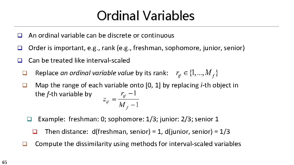
Ordinal Variables q An ordinal variable can be discrete or continuous q Order is important, e. g. , rank (e. g. , freshman, sophomore, junior, senior) q Can be treated like interval-scaled q Replace an ordinal variable value by its rank: q Map the range of each variable onto [0, 1] by replacing i-th object in the f-th variable by Example: freshman: 0; sophomore: 1/3; junior: 2/3; senior 1 q q q 65 Then distance: d(freshman, senior) = 1, d(junior, senior) = 1/3 Compute the dissimilarity using methods for interval-scaled variables

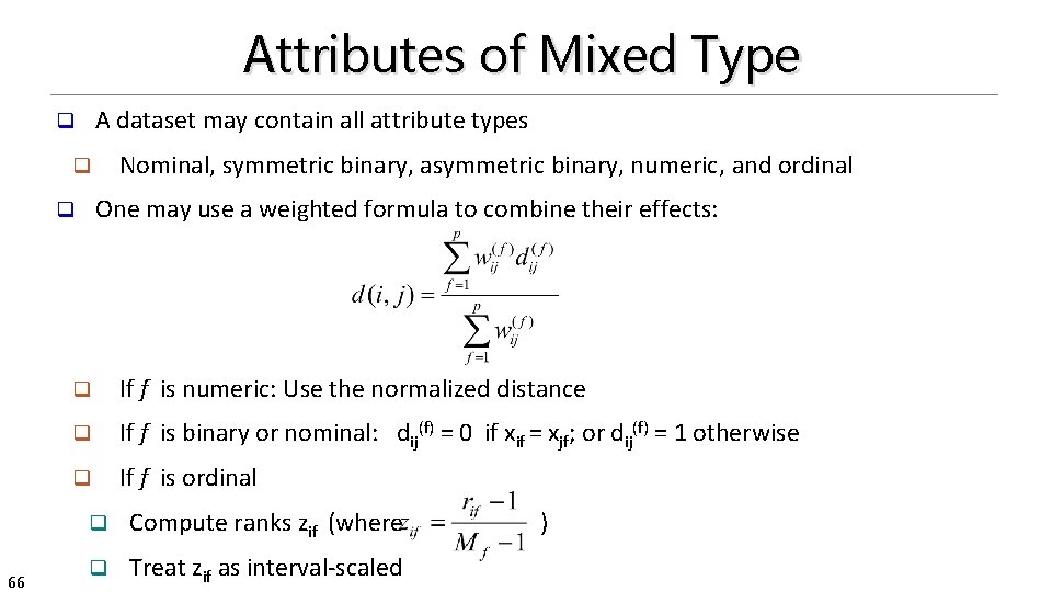
Attributes of Mixed Type A dataset may contain all attribute types q Nominal, symmetric binary, asymmetric binary, numeric, and ordinal q One may use a weighted formula to combine their effects: q 66 q If f is numeric: Use the normalized distance q If f is binary or nominal: dij(f) = 0 if xif = xjf; or dij(f) = 1 otherwise q If f is ordinal q Compute ranks zif (where q Treat zif as interval-scaled )

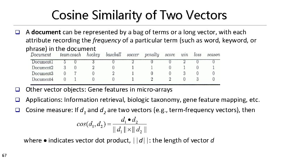
Cosine Similarity of Two Vectors q A document can be represented by a bag of terms or a long vector, with each attribute recording the frequency of a particular term (such as word, keyword, or phrase) in the document Other vector objects: Gene features in micro-arrays q Applications: Information retrieval, biologic taxonomy, gene feature mapping, etc. q Cosine measure: If d 1 and d 2 are two vectors (e. g. , term-frequency vectors), then q where indicates vector dot product, ||d||: the length of vector d 67

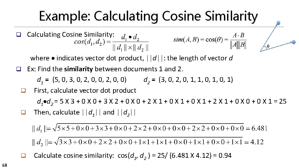
Example: Calculating Cosine Similarity q Calculating Cosine Similarity: where indicates vector dot product, ||d||: the length of vector d q Ex: Find the similarity between documents 1 and 2. d 1 = (5, 0, 3, 0, 2, 0, 0) d 2 = (3, 0, 2, 0, 1, 1, 0, 1) q First, calculate vector dot product d 1 d 2 = 5 X 3 + 0 X 0 + 3 X 2 + 0 X 0 + 2 X 1 + 0 X 1 + 2 X 1 + 0 X 0 + 0 X 1 = 25 q Then, calculate ||d 1|| and ||d 2|| q 68 Calculate cosine similarity: cos(d 1, d 2 ) = 25/ (6. 481 X 4. 12) = 0. 94

Announcements: Meetine of the 4 th Credit Project CS 412: Assignment #1 was distributed last Tuesday! q The due date is Sept. 15. No late homework will be accepted!! q Waitlist is cleared: We took 50 additional students into the video only session q Please find your status with Holly. You are either in or out (wait for Spring 2017) q Meeting for Project for the 4 th Credit q You can change from 4 to 3 credit or from 3 to 4 credits by sending me e-mails q Meeting time and location: 10 -11 am Friday (tomorrow!) at 0216 SC q This project is part of WSDM 2017 Cup q Choice #1: Triple Scoring: Computing relevance scores for triples from type-like relations q Choice #2: Vandalism Detection for Wikipages q Tas/Ph. D student/postdoc will give you the details in the Friday meeting! Must attend if you want to do the 4 th credit project!!! q 69

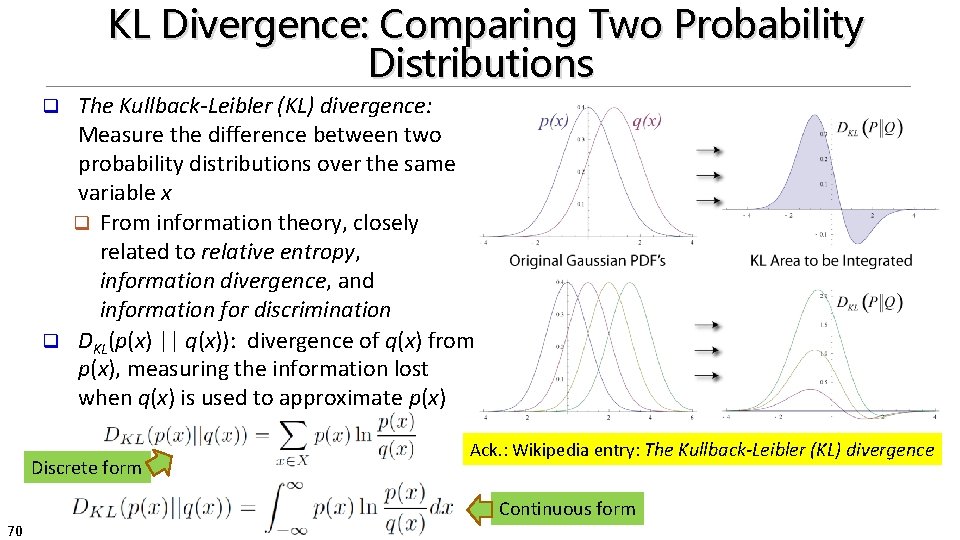
KL Divergence: Comparing Two Probability Distributions The Kullback-Leibler (KL) divergence: Measure the difference between two probability distributions over the same variable x q From information theory, closely related to relative entropy, information divergence, and information for discrimination q DKL(p(x) || q(x)): divergence of q(x) from p(x), measuring the information lost when q(x) is used to approximate p(x) q Discrete form Ack. : Wikipedia entry: The Kullback-Leibler (KL) divergence Continuous form 70

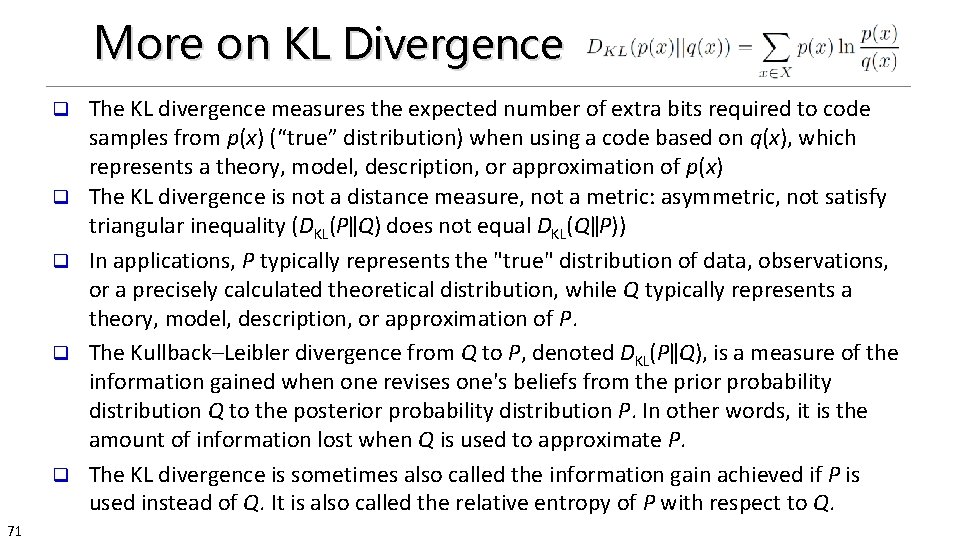
More on KL Divergence q q q 71 The KL divergence measures the expected number of extra bits required to code samples from p(x) (“true” distribution) when using a code based on q(x), which represents a theory, model, description, or approximation of p(x) The KL divergence is not a distance measure, not a metric: asymmetric, not satisfy triangular inequality (DKL(P‖Q) does not equal DKL(Q‖P)) In applications, P typically represents the "true" distribution of data, observations, or a precisely calculated theoretical distribution, while Q typically represents a theory, model, description, or approximation of P. The Kullback–Leibler divergence from Q to P, denoted DKL(P‖Q), is a measure of the information gained when one revises one's beliefs from the prior probability distribution Q to the posterior probability distribution P. In other words, it is the amount of information lost when Q is used to approximate P. The KL divergence is sometimes also called the information gain achieved if P is used instead of Q. It is also called the relative entropy of P with respect to Q.

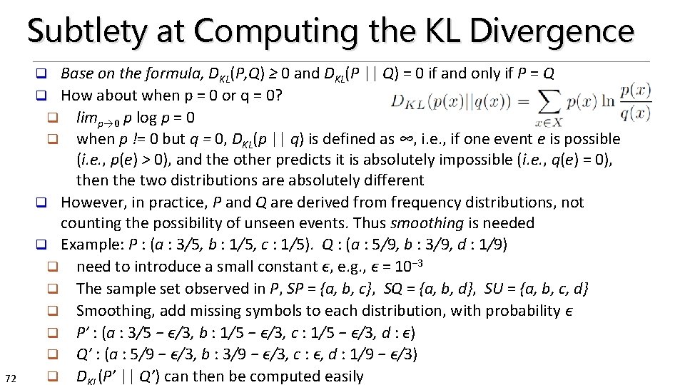
Subtlety at Computing the KL Divergence Base on the formula, DKL(P, Q) ≥ 0 and DKL(P || Q) = 0 if and only if P = Q q How about when p = 0 or q = 0? q limp→ 0 p log p = 0 q when p != 0 but q = 0, DKL(p || q) is defined as ∞, i. e. , if one event e is possible (i. e. , p(e) > 0), and the other predicts it is absolutely impossible (i. e. , q(e) = 0), then the two distributions are absolutely different q However, in practice, P and Q are derived from frequency distributions, not counting the possibility of unseen events. Thus smoothing is needed q Example: P : (a : 3/5, b : 1/5, c : 1/5). Q : (a : 5/9, b : 3/9, d : 1/9) q need to introduce a small constant ϵ, e. g. , ϵ = 10− 3 q The sample set observed in P, SP = {a, b, c}, SQ = {a, b, d}, SU = {a, b, c, d} q Smoothing, add missing symbols to each distribution, with probability ϵ q P′ : (a : 3/5 − ϵ/3, b : 1/5 − ϵ/3, c : 1/5 − ϵ/3, d : ϵ) q Q′ : (a : 5/9 − ϵ/3, b : 3/9 − ϵ/3, c : ϵ, d : 1/9 − ϵ/3) q D (P’ || Q’) can then be computed easily q 72

Chapter 2. Getting to Know Your Data 73 q Data Objects and Attribute Types q Basic Statistical Descriptions of Data q Data Visualization q Measuring Data Similarity and Dissimilarity q Summary

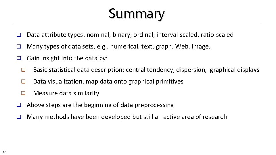
Summary 74 q Data attribute types: nominal, binary, ordinal, interval-scaled, ratio-scaled q Many types of data sets, e. g. , numerical, text, graph, Web, image. q Gain insight into the data by: q Basic statistical data description: central tendency, dispersion, graphical displays q Data visualization: map data onto graphical primitives q Measure data similarity q Above steps are the beginning of data preprocessing q Many methods have been developed but still an active area of research

References q q q q q 75 W. Cleveland, Visualizing Data, Hobart Press, 1993 T. Dasu and T. Johnson. Exploratory Data Mining and Data Cleaning. John Wiley, 2003 U. Fayyad, G. Grinstein, and A. Wierse. Information Visualization in Data Mining and Knowledge Discovery, Morgan Kaufmann, 2001 L. Kaufman and P. J. Rousseeuw. Finding Groups in Data: an Introduction to Cluster Analysis. John Wiley & Sons, 1990. H. V. Jagadish et al. , Special Issue on Data Reduction Techniques. Bulletin of the Tech. Committee on Data Eng. , 20(4), Dec. 1997 D. A. Keim. Information visualization and visual data mining, IEEE trans. on Visualization and Computer Graphics, 8(1), 2002 D. Pyle. Data Preparation for Data Mining. Morgan Kaufmann, 1999 S. Santini and R. Jain, ” Similarity measures”, IEEE Trans. on Pattern Analysis and Machine Intelligence, 21(9), 1999 E. R. Tufte. The Visual Display of Quantitative Information, 2 nd ed. , Graphics Press, 2001 C. Yu, et al. , Visual data mining of multimedia data for social and behavioral studies, Information Visualization, 8(1), 2009

76 February 10, 2022 Data Mining: Concepts and Techniques 76