CS 267 Lecture 2 Single Processor Machines Memory

CS 267 Lecture 2 Single Processor Machines: Memory Hierarchies and Processor Features Case Study: Tuning Matrix Multiply James Demmel http: //www. cs. berkeley. edu/~demmel/cs 267_Spr 12/ 1

Motivation • Most applications run at < 10% of the “peak” performance of a system • Peak is the maximum the hardware can physically execute • Much of this performance is lost on a single processor, i. e. , the code running on one processor often runs at only 1020% of the processor peak • Most of the single processor performance loss is in the memory system • Moving data takes much longer than arithmetic and logic • To understand this, we need to look under the hood of modern processors • For today, we will look at only a single “core” processor • These issues will exist on processors within any parallel computer 01/19/2012 CS 267 - Lecture 2 2

Possible conclusions to draw from today’s lecture • “Computer architectures are fascinating, and I really want to understand why apparently simple programs can behave in such complex ways!” • “I want to learn how to design algorithms that run really fast no matter how complicated the underlying computer architecture. ” • “I hope that most of the time I can use fast software that someone else has written and hidden all these details from me so I don’t have to worry about them!” • All of the above, at different points in time 01/19/2012 CS 267 - Lecture 2 3

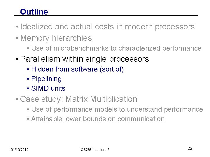
Outline • Idealized and actual costs in modern processors • Memory hierarchies • Use of microbenchmarks to characterized performance • Parallelism within single processors • Case study: Matrix Multiplication • Use of performance models to understand performance • Attainable lower bounds on communication 01/19/2012 CS 267 - Lecture 2 4

Outline • Idealized and actual costs in modern processors • Memory hierarchies • Use of microbenchmarks to characterized performance • Parallelism within single processors • Case study: Matrix Multiplication • Use of performance models to understand performance • Attainable lower bounds on communication 01/19/2012 CS 267 - Lecture 2 5

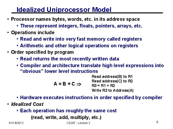
Idealized Uniprocessor Model • Processor names bytes, words, etc. in its address space • These represent integers, floats, pointers, arrays, etc. • Operations include • Read and write into very fast memory called registers • Arithmetic and other logical operations on registers • Order specified by program • Read returns the most recently written data • Compiler and architecture translate high level expressions into “obvious” lower level instructions A=B+C Read address(B) to R 1 Read address(C) to R 2 R 3 = R 1 + R 2 Write R 3 to Address(A) • Hardware executes instructions in order specified by compiler • Idealized Cost • Each operation has roughly the same cost (read, write, add, multiply, etc. ) 01/19/2012 CS 267 - Lecture 2 6

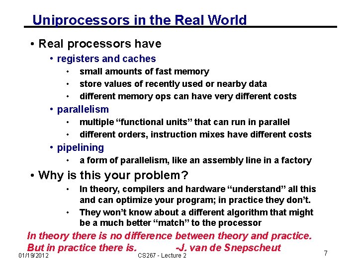
Uniprocessors in the Real World • Real processors have • registers and caches • • • small amounts of fast memory store values of recently used or nearby data different memory ops can have very different costs • parallelism • • multiple “functional units” that can run in parallel different orders, instruction mixes have different costs • pipelining • a form of parallelism, like an assembly line in a factory • Why is this your problem? • • In theory, compilers and hardware “understand” all this and can optimize your program; in practice they don’t. They won’t know about a different algorithm that might be a much better “match” to the processor In theory there is no difference between theory and practice. But in practice there is. -J. van de Snepscheut 01/19/2012 CS 267 - Lecture 2 7

Outline • Idealized and actual costs in modern processors • Memory hierarchies • Temporal and spatial locality • Basics of caches • Use of microbenchmarks to characterized performance • Parallelism within single processors • Case study: Matrix Multiplication • Use of performance models to understand performance • Attainable lower bounds on communication 01/19/2012 CS 267 - Lecture 2 8

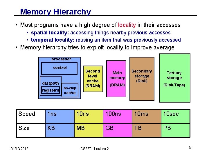
Memory Hierarchy • Most programs have a high degree of locality in their accesses • spatial locality: accessing things nearby previous accesses • temporal locality: reusing an item that was previously accessed • Memory hierarchy tries to exploit locality to improve average processor control Second level cache (SRAM) datapath registers on-chip Main memory (DRAM) Secondary storage (Disk) Tertiary storage (Disk/Tape) cache Speed 1 ns 100 ns 10 ms 10 sec Size KB MB GB TB PB 01/19/2012 CS 267 - Lecture 2 9

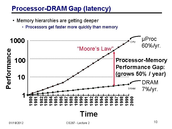
Processor-DRAM Gap (latency) • Memory hierarchies are getting deeper • Processors get faster more quickly than memory CPU “Moore’s Law” 100 Processor-Memory Performance Gap: (grows 50% / year) DRAM 7%/yr. 10 1 µProc 60%/yr. 1980 1981 1982 1983 1984 1985 1986 1987 1988 1989 1990 1991 1992 1993 1994 1995 1996 1997 1998 1999 2000 Performance 1000 Time 01/19/2012 CS 267 - Lecture 2 10

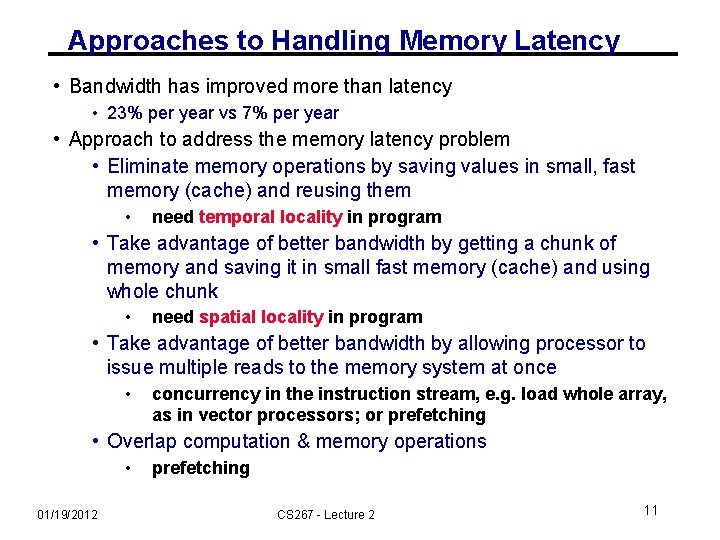
Approaches to Handling Memory Latency • Bandwidth has improved more than latency • 23% per year vs 7% per year • Approach to address the memory latency problem • Eliminate memory operations by saving values in small, fast memory (cache) and reusing them • need temporal locality in program • Take advantage of better bandwidth by getting a chunk of memory and saving it in small fast memory (cache) and using whole chunk • need spatial locality in program • Take advantage of better bandwidth by allowing processor to issue multiple reads to the memory system at once • concurrency in the instruction stream, e. g. load whole array, as in vector processors; or prefetching • Overlap computation & memory operations • 01/19/2012 prefetching CS 267 - Lecture 2 11

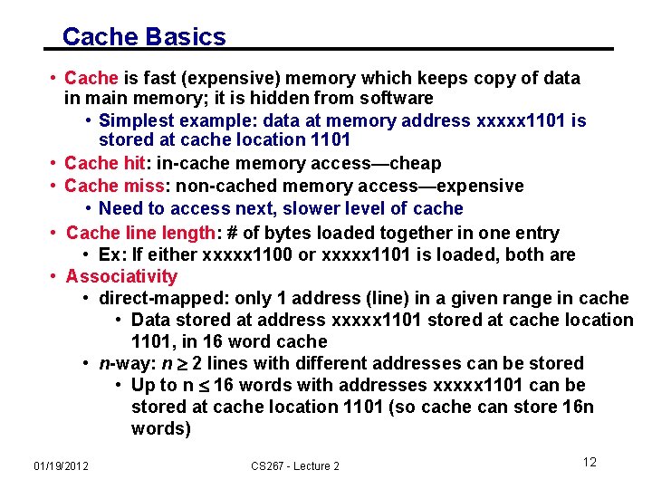
Cache Basics • Cache is fast (expensive) memory which keeps copy of data in main memory; it is hidden from software • Simplest example: data at memory address xxxxx 1101 is stored at cache location 1101 • Cache hit: in-cache memory access—cheap • Cache miss: non-cached memory access—expensive • Need to access next, slower level of cache • Cache line length: # of bytes loaded together in one entry • Ex: If either xxxxx 1100 or xxxxx 1101 is loaded, both are • Associativity • direct-mapped: only 1 address (line) in a given range in cache • Data stored at address xxxxx 1101 stored at cache location 1101, in 16 word cache • n-way: n 2 lines with different addresses can be stored • Up to n 16 words with addresses xxxxx 1101 can be stored at cache location 1101 (so cache can store 16 n words) 01/19/2012 CS 267 - Lecture 2 12

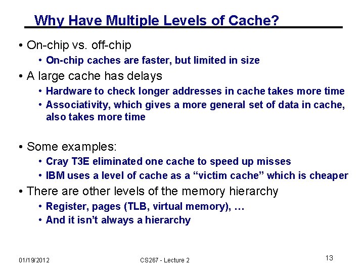
Why Have Multiple Levels of Cache? • On-chip vs. off-chip • On-chip caches are faster, but limited in size • A large cache has delays • Hardware to check longer addresses in cache takes more time • Associativity, which gives a more general set of data in cache, also takes more time • Some examples: • Cray T 3 E eliminated one cache to speed up misses • IBM uses a level of cache as a “victim cache” which is cheaper • There are other levels of the memory hierarchy • Register, pages (TLB, virtual memory), … • And it isn’t always a hierarchy 01/19/2012 CS 267 - Lecture 2 13

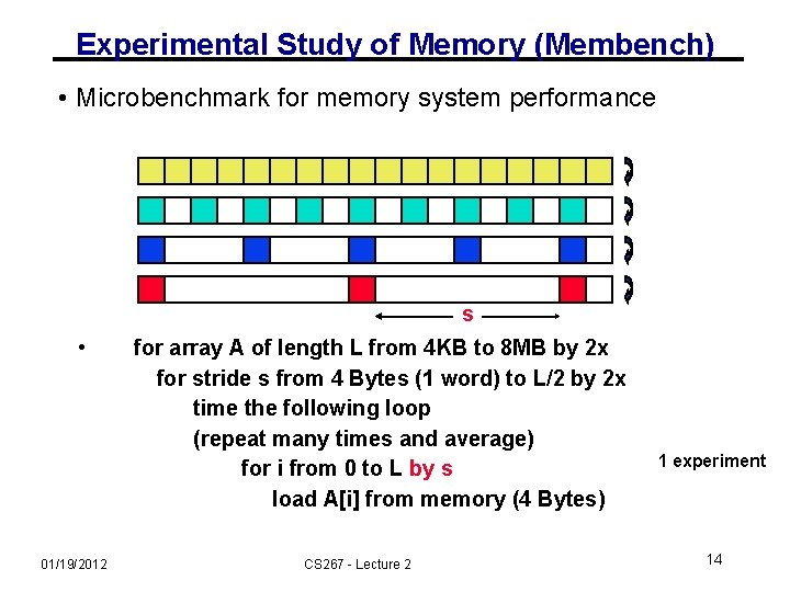
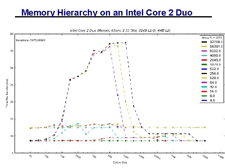
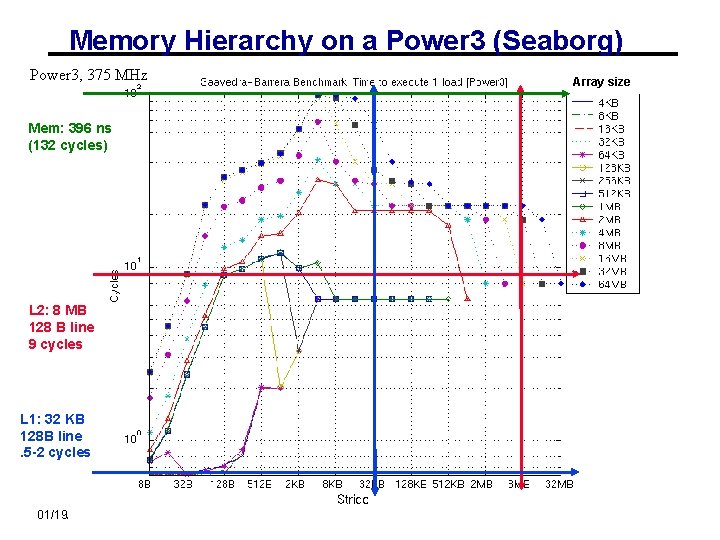
Experimental Study of Memory (Membench) • Microbenchmark for memory system performance s • 01/19/2012 for array A of length L from 4 KB to 8 MB by 2 x for stride s from 4 Bytes (1 word) to L/2 by 2 x time the following loop (repeat many times and average) for i from 0 to L by s load A[i] from memory (4 Bytes) CS 267 - Lecture 2 1 experiment 14

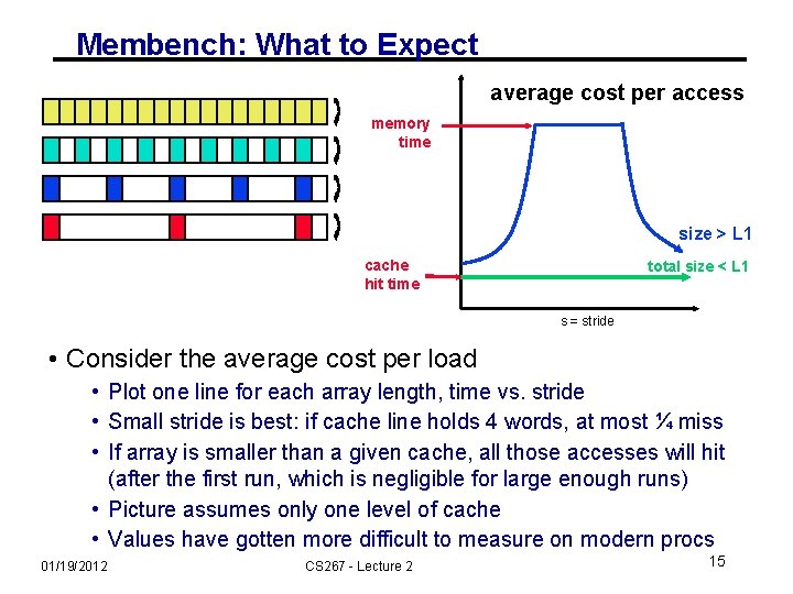
Membench: What to Expect average cost per access memory time size > L 1 cache hit time total size < L 1 s = stride • Consider the average cost per load • Plot one line for each array length, time vs. stride • Small stride is best: if cache line holds 4 words, at most ¼ miss • If array is smaller than a given cache, all those accesses will hit (after the first run, which is negligible for large enough runs) • Picture assumes only one level of cache • Values have gotten more difficult to measure on modern procs 01/19/2012 CS 267 - Lecture 2 15

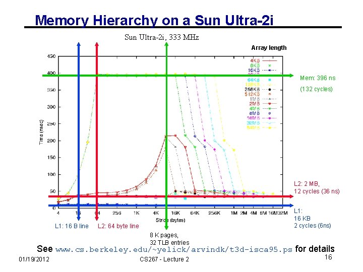
Memory Hierarchy on a Sun Ultra-2 i, 333 MHz Array length Mem: 396 ns (132 cycles) L 2: 2 MB, 12 cycles (36 ns) L 1: 16 B line L 1: 16 KB 2 cycles (6 ns) L 2: 64 byte line 8 K pages, 32 TLB entries See www. cs. berkeley. edu/~yelick/arvindk/t 3 d-isca 95. ps for details 01/19/2012 CS 267 - Lecture 2 16

Memory Hierarchy on an Intel Core 2 Duo 01/19/2012 CS 267 - Lecture 2 17

Memory Hierarchy on a Power 3 (Seaborg) Power 3, 375 MHz Array size Mem: 396 ns (132 cycles) L 2: 8 MB 128 B line 9 cycles L 1: 32 KB 128 B line. 5 -2 cycles 01/19/2012 CS 267 - Lecture 2 18

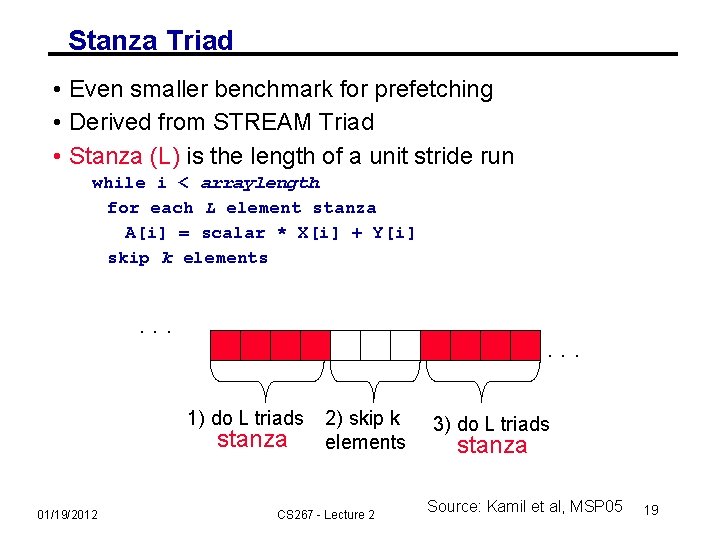
Stanza Triad • Even smaller benchmark for prefetching • Derived from STREAM Triad • Stanza (L) is the length of a unit stride run while i < arraylength for each L element stanza A[i] = scalar * X[i] + Y[i] skip k elements . . . 1) do L triads stanza 01/19/2012 2) skip k elements CS 267 - Lecture 2 3) do L triads stanza Source: Kamil et al, MSP 05 19

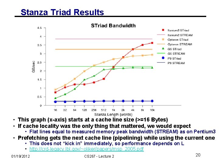
Stanza Triad Results • This graph (x-axis) starts at a cache line size (>=16 Bytes) • If cache locality was the only thing that mattered, we would expect • Flat lines equal to measured memory peak bandwidth (STREAM) as on Pentium 3 • Prefetching gets the next cache line (pipelining) while using the current one • This does not “kick in” immediately, so performance depends on L • http: //crd-legacy. lbl. gov/~oliker/papers/msp_2005. pdf 01/19/2012 CS 267 - Lecture 2 20

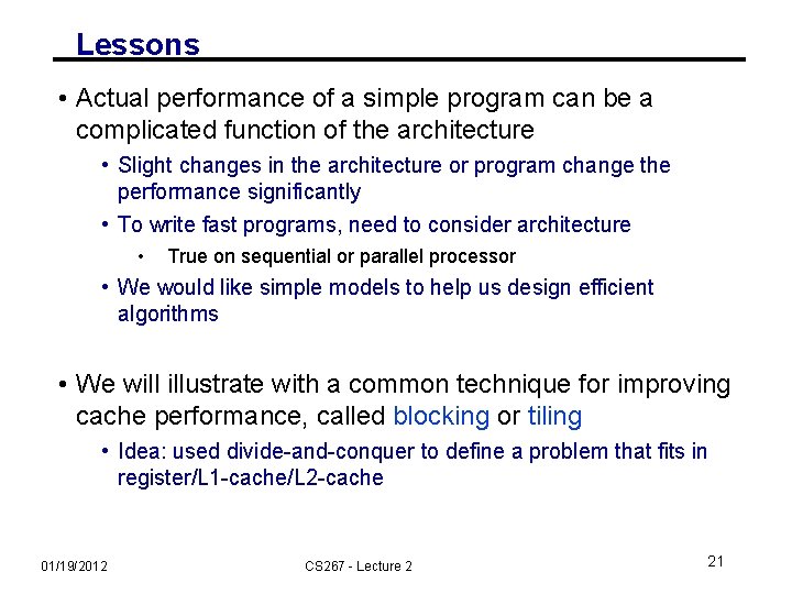
Lessons • Actual performance of a simple program can be a complicated function of the architecture • Slight changes in the architecture or program change the performance significantly • To write fast programs, need to consider architecture • True on sequential or parallel processor • We would like simple models to help us design efficient algorithms • We will illustrate with a common technique for improving cache performance, called blocking or tiling • Idea: used divide-and-conquer to define a problem that fits in register/L 1 -cache/L 2 -cache 01/19/2012 CS 267 - Lecture 2 21

Outline • Idealized and actual costs in modern processors • Memory hierarchies • Use of microbenchmarks to characterized performance • Parallelism within single processors • Hidden from software (sort of) • Pipelining • SIMD units • Case study: Matrix Multiplication • Use of performance models to understand performance • Attainable lower bounds on communication 01/19/2012 CS 267 - Lecture 2 22

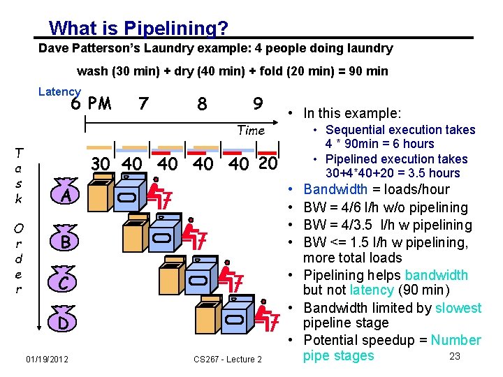
What is Pipelining? Dave Patterson’s Laundry example: 4 people doing laundry wash (30 min) + dry (40 min) + fold (20 min) = 90 min Latency 6 PM 7 8 9 • In this example: Time T a s k O r d e r • Sequential execution takes 4 * 90 min = 6 hours • Pipelined execution takes 30+4*40+20 = 3. 5 hours 30 40 40 20 • • A B C D 01/19/2012 CS 267 - Lecture 2 Bandwidth = loads/hour BW = 4/6 l/h w/o pipelining BW = 4/3. 5 l/h w pipelining BW <= 1. 5 l/h w pipelining, more total loads • Pipelining helps bandwidth but not latency (90 min) • Bandwidth limited by slowest pipeline stage • Potential speedup = Number 23 pipe stages

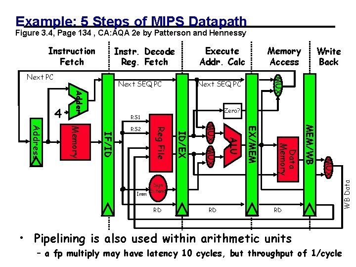
Example: 5 Steps of MIPS Datapath Figure 3. 4, Page 134 , CA: AQA 2 e by Patterson and Hennessy Execute Addr. Calc Instr. Decode Reg. Fetch Next SEQ PC Adder 4 Zero? RS 1 RD RD RD MUX Sign Extend MEM/WB Data Memory EX/MEM ALU MUX ID/EX Imm Reg File IF/ID Memory Address RS 2 Write Back MUX Next PC Memory Access WB Data Instruction Fetch • Pipelining is also used within arithmetic units – a 01/19/2012 24 fp multiply may have latency cycles, but throughput of 1/cycle CS 267 - Lecture 10 2

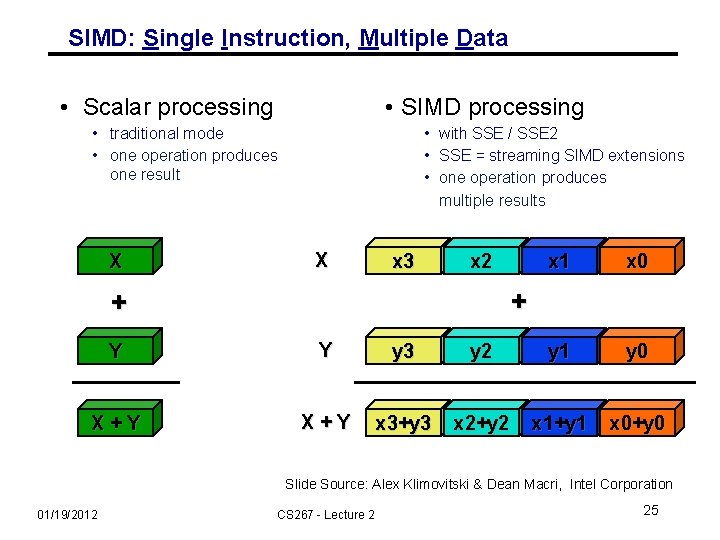
SIMD: Single Instruction, Multiple Data • Scalar processing • SIMD processing • traditional mode • one operation produces one result X • with SSE / SSE 2 • SSE = streaming SIMD extensions • one operation produces multiple results X x 3 x 2 x 1 x 0 + + Y Y y 3 y 2 y 1 y 0 X+Y x 3+y 3 x 2+y 2 x 1+y 1 x 0+y 0 Slide Source: Alex Klimovitski & Dean Macri, Intel Corporation 01/19/2012 CS 267 - Lecture 2 25

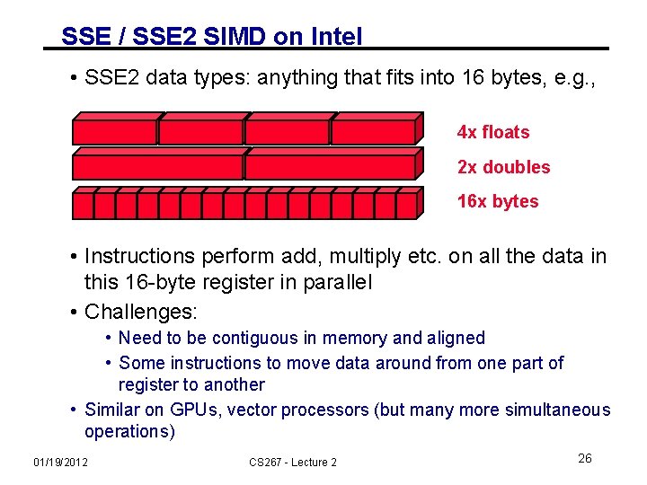
SSE / SSE 2 SIMD on Intel • SSE 2 data types: anything that fits into 16 bytes, e. g. , 4 x floats 2 x doubles 16 x bytes • Instructions perform add, multiply etc. on all the data in this 16 -byte register in parallel • Challenges: • Need to be contiguous in memory and aligned • Some instructions to move data around from one part of register to another • Similar on GPUs, vector processors (but many more simultaneous operations) 01/19/2012 CS 267 - Lecture 2 26

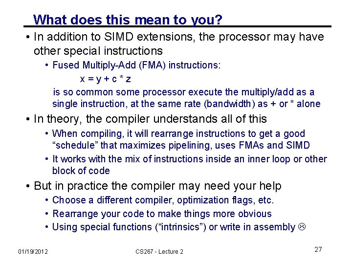
What does this mean to you? • In addition to SIMD extensions, the processor may have other special instructions • Fused Multiply-Add (FMA) instructions: x=y+c*z is so common some processor execute the multiply/add as a single instruction, at the same rate (bandwidth) as + or * alone • In theory, the compiler understands all of this • When compiling, it will rearrange instructions to get a good “schedule” that maximizes pipelining, uses FMAs and SIMD • It works with the mix of instructions inside an inner loop or other block of code • But in practice the compiler may need your help • Choose a different compiler, optimization flags, etc. • Rearrange your code to make things more obvious • Using special functions (“intrinsics”) or write in assembly 01/19/2012 CS 267 - Lecture 2 27

Outline • Idealized and actual costs in modern processors • Memory hierarchies • Use of microbenchmarks to characterized performance • Parallelism within single processors • Case study: Matrix Multiplication • Use of performance models to understand performance • Attainable lower bounds on communication • Simple cache model • Warm-up: Matrix-vector multiplication • Naïve vs optimized Matrix-Matrix Multiply • Minimizing data movement • Beating O(n 3) operations • Practical optimizations (continued next time) 01/19/2012 CS 267 - Lecture 2 28

Why Matrix Multiplication? • An important kernel in many problems • Appears in many linear algebra algorithms • Bottleneck for dense linear algebra • One of the 7 dwarfs / 13 motifs of parallel computing • Closely related to other algorithms, e. g. , transitive closure on a graph using Floyd-Warshall • Optimization ideas can be used in other problems • The best case for optimization payoffs • The most-studied algorithm in high performance computing 01/19/2012 CS 267 - Lecture 2 29

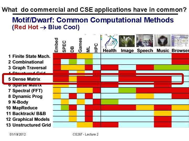
What do commercial and CSE applications have in common? Motif/Dwarf: Common Computational Methods (Red Hot Blue Cool) 01/19/2012 CS 267 - Lecture 2

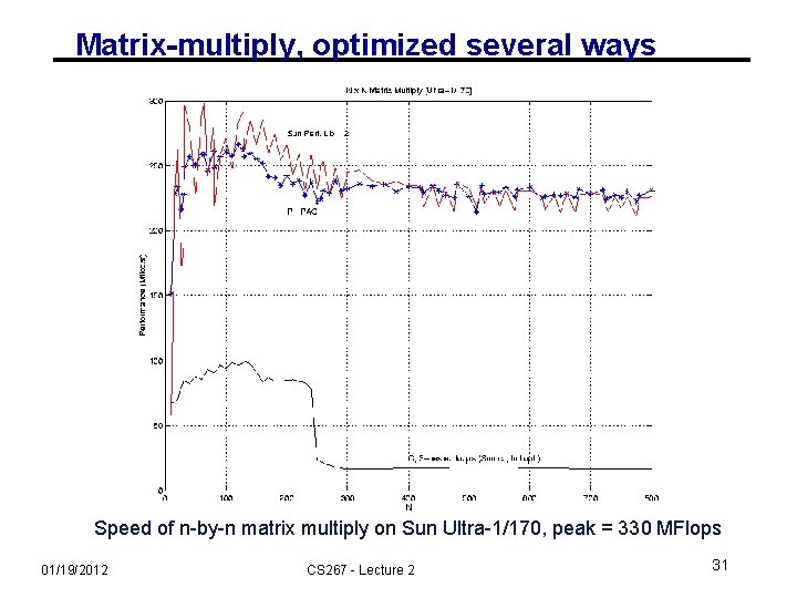
Matrix-multiply, optimized several ways Speed of n-by-n matrix multiply on Sun Ultra-1/170, peak = 330 MFlops 01/19/2012 CS 267 - Lecture 2 31

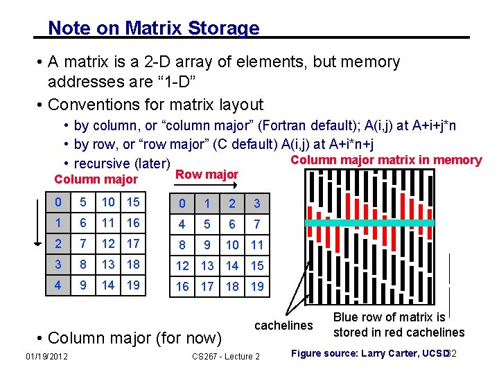
Note on Matrix Storage • A matrix is a 2 -D array of elements, but memory addresses are “ 1 -D” • Conventions for matrix layout • by column, or “column major” (Fortran default); A(i, j) at A+i+j*n • by row, or “row major” (C default) A(i, j) at A+i*n+j Column major matrix in memory • recursive (later) Column major Row major 0 5 10 15 0 1 2 3 1 6 11 16 4 5 6 7 2 7 12 17 8 9 10 11 3 8 13 18 12 13 14 15 4 9 14 19 16 17 18 19 • Column major (for now) 01/19/2012 cachelines CS 267 - Lecture 2 Blue row of matrix is stored in red cachelines Figure source: Larry Carter, UCSD 32

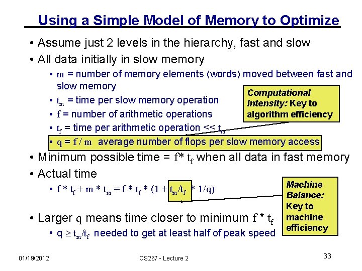
Using a Simple Model of Memory to Optimize • Assume just 2 levels in the hierarchy, fast and slow • All data initially in slow memory • m = number of memory elements (words) moved between fast and slow memory Computational • tm = time per slow memory operation Intensity: Key to • f = number of arithmetic operations algorithm efficiency • tf = time per arithmetic operation << tm • q = f / m average number of flops per slow memory access • Minimum possible time = f* tf when all data in fast memory • Actual time • f * tf + m * tm = f * tf * (1 + tm/tf * 1/q) • Larger q means time closer to minimum f * tf • q tm/tf needed to get at least half of peak speed 01/19/2012 CS 267 - Lecture 2 Machine Balance: Key to machine efficiency 33

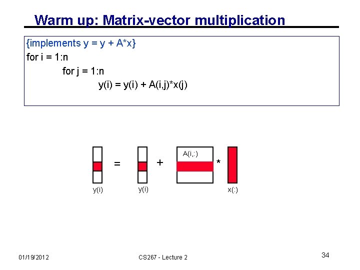
Warm up: Matrix-vector multiplication {implements y = y + A*x} for i = 1: n for j = 1: n y(i) = y(i) + A(i, j)*x(j) + = y(i) 01/19/2012 A(i, : ) y(i) CS 267 - Lecture 2 * x(: ) 34

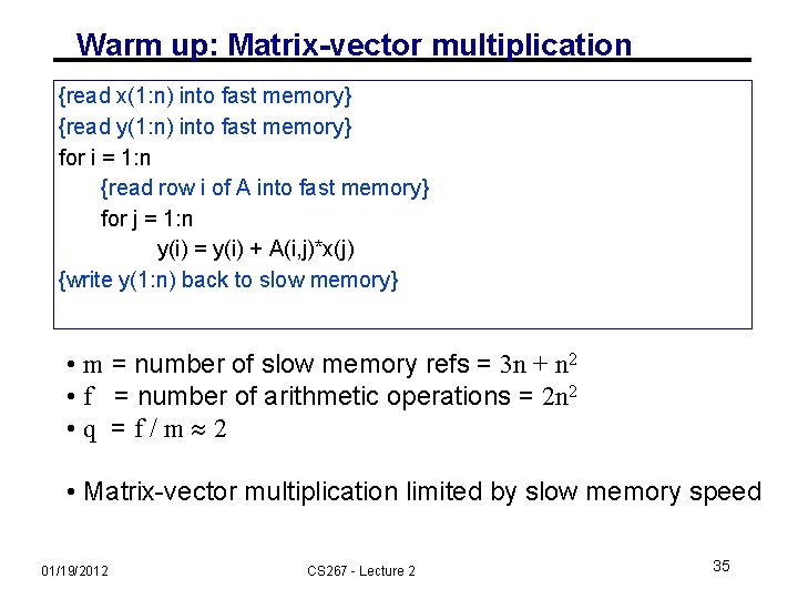
Warm up: Matrix-vector multiplication {read x(1: n) into fast memory} {read y(1: n) into fast memory} for i = 1: n {read row i of A into fast memory} for j = 1: n y(i) = y(i) + A(i, j)*x(j) {write y(1: n) back to slow memory} • m = number of slow memory refs = 3 n + n 2 • f = number of arithmetic operations = 2 n 2 • q =f/m 2 • Matrix-vector multiplication limited by slow memory speed 01/19/2012 CS 267 - Lecture 2 35

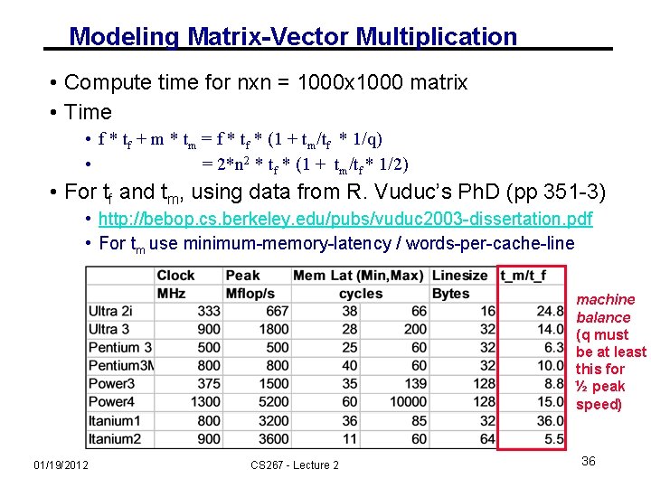
Modeling Matrix-Vector Multiplication • Compute time for nxn = 1000 x 1000 matrix • Time • f * tf + m * tm = f * tf * (1 + tm/tf * 1/q) • = 2*n 2 * tf * (1 + tm/tf * 1/2) • For tf and tm, using data from R. Vuduc’s Ph. D (pp 351 -3) • http: //bebop. cs. berkeley. edu/pubs/vuduc 2003 -dissertation. pdf • For tm use minimum-memory-latency / words-per-cache-line machine balance (q must be at least this for ½ peak speed) 01/19/2012 CS 267 - Lecture 2 36

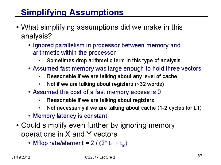
Simplifying Assumptions • What simplifying assumptions did we make in this analysis? • Ignored parallelism in processor between memory and arithmetic within the processor • Sometimes drop arithmetic term in this type of analysis • Assumed fast memory was large enough to hold three vectors • • Reasonable if we are talking about any level of cache Not if we are talking about registers (~32 words) • Assumed the cost of a fast memory access is 0 • • Reasonable if we are talking about registers Not necessarily if we are talking about cache (1 -2 cycles for L 1) • Memory latency is constant • Could simplify even further by ignoring memory operations in X and Y vectors • Mflop rate/element = 2 / (2* tf + tm) 01/19/2012 CS 267 - Lecture 2 37

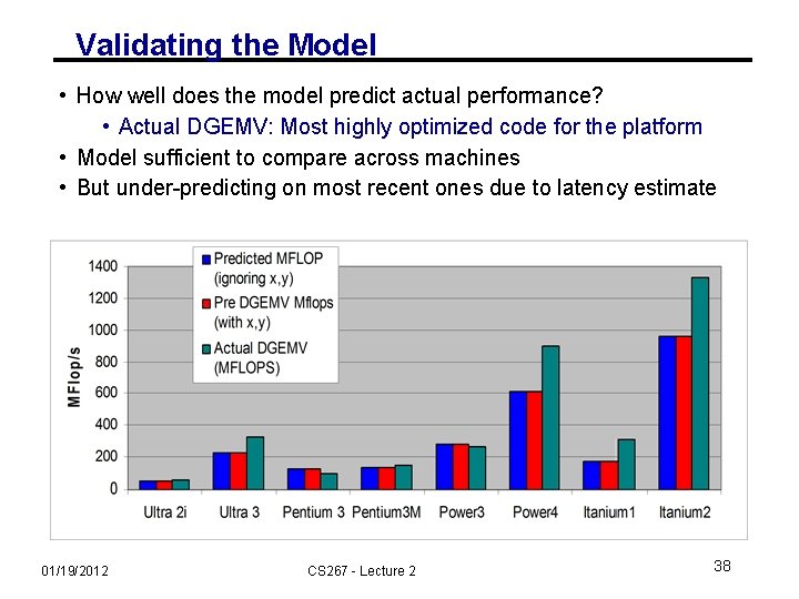
Validating the Model • How well does the model predict actual performance? • Actual DGEMV: Most highly optimized code for the platform • Model sufficient to compare across machines • But under-predicting on most recent ones due to latency estimate 01/19/2012 CS 267 - Lecture 2 38

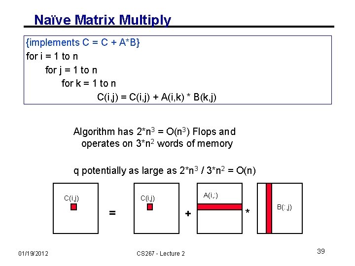
Naïve Matrix Multiply {implements C = C + A*B} for i = 1 to n for j = 1 to n for k = 1 to n C(i, j) = C(i, j) + A(i, k) * B(k, j) Algorithm has 2*n 3 = O(n 3) Flops and operates on 3*n 2 words of memory q potentially as large as 2*n 3 / 3*n 2 = O(n) C(i, j) = 01/19/2012 A(i, : ) C(i, j) + CS 267 - Lecture 2 * B(: , j) 39

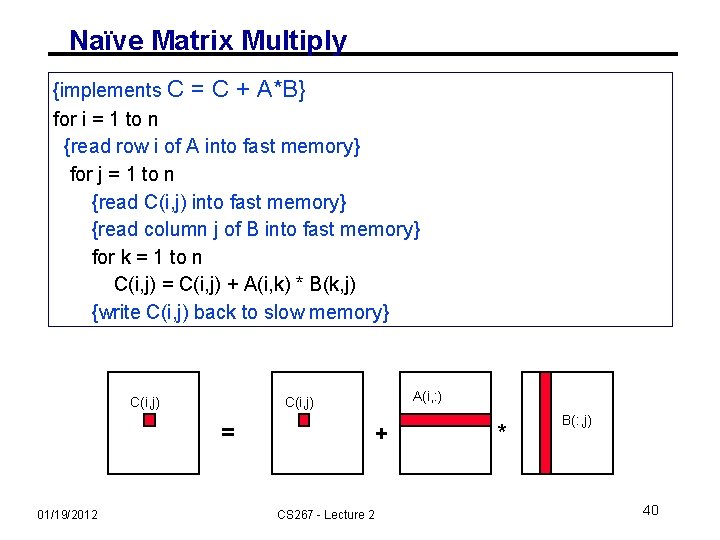
Naïve Matrix Multiply {implements C = C + A*B} for i = 1 to n {read row i of A into fast memory} for j = 1 to n {read C(i, j) into fast memory} {read column j of B into fast memory} for k = 1 to n C(i, j) = C(i, j) + A(i, k) * B(k, j) {write C(i, j) back to slow memory} C(i, j) = 01/19/2012 A(i, : ) C(i, j) + CS 267 - Lecture 2 * B(: , j) 40

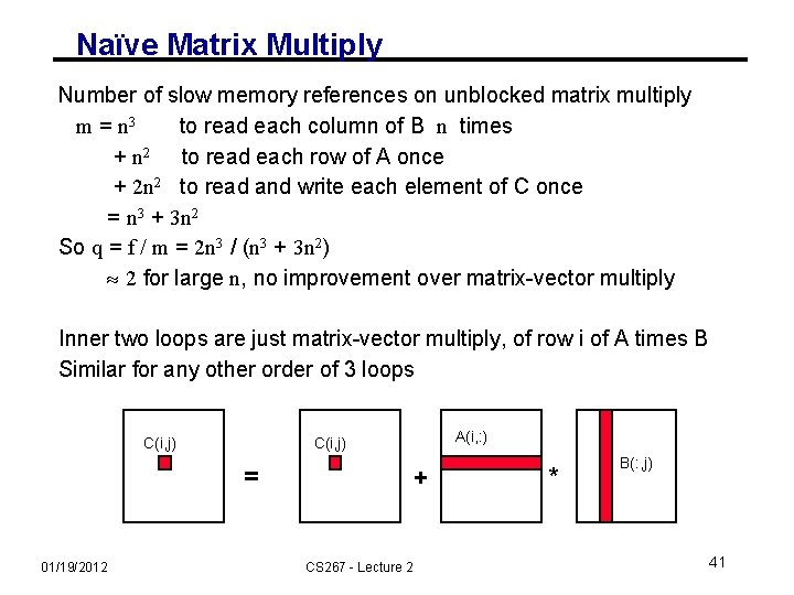
Naïve Matrix Multiply Number of slow memory references on unblocked matrix multiply m = n 3 to read each column of B n times + n 2 to read each row of A once + 2 n 2 to read and write each element of C once = n 3 + 3 n 2 So q = f / m = 2 n 3 / (n 3 + 3 n 2) 2 for large n, no improvement over matrix-vector multiply Inner two loops are just matrix-vector multiply, of row i of A times B Similar for any other order of 3 loops C(i, j) = 01/19/2012 A(i, : ) C(i, j) + CS 267 - Lecture 2 * B(: , j) 41

Matrix-multiply, optimized several ways Speed of n-by-n matrix multiply on Sun Ultra-1/170, peak = 330 MFlops 01/19/2012 CS 267 - Lecture 2 42

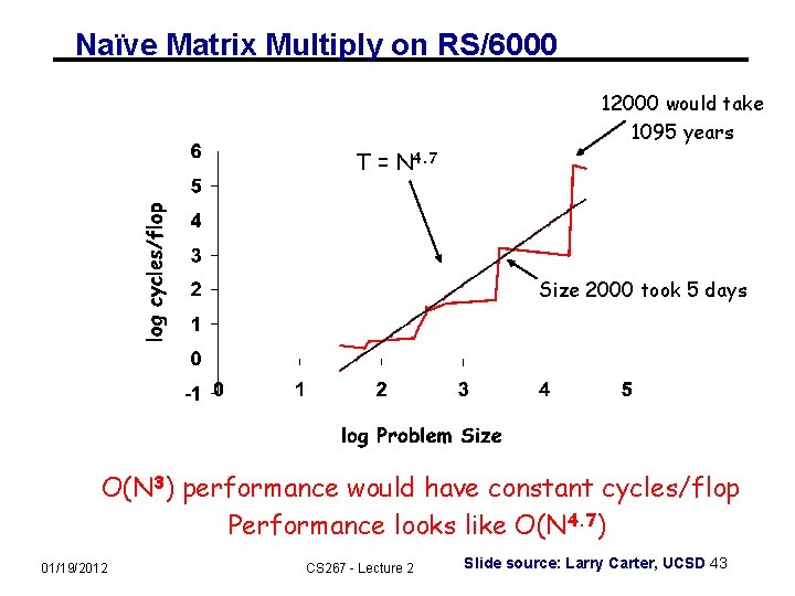
Naïve Matrix Multiply on RS/6000 12000 would take 1095 years T = N 4. 7 Size 2000 took 5 days O(N 3) performance would have constant cycles/flop Performance looks like O(N 4. 7) 01/19/2012 CS 267 - Lecture 2 Slide source: Larry Carter, UCSD 43

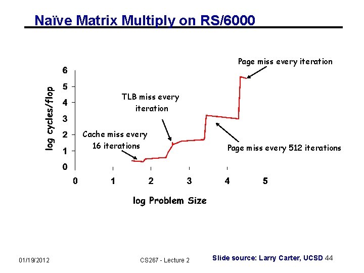
Naïve Matrix Multiply on RS/6000 Page miss every iteration TLB miss every iteration Cache miss every 16 iterations 01/19/2012 CS 267 - Lecture 2 Page miss every 512 iterations Slide source: Larry Carter, UCSD 44

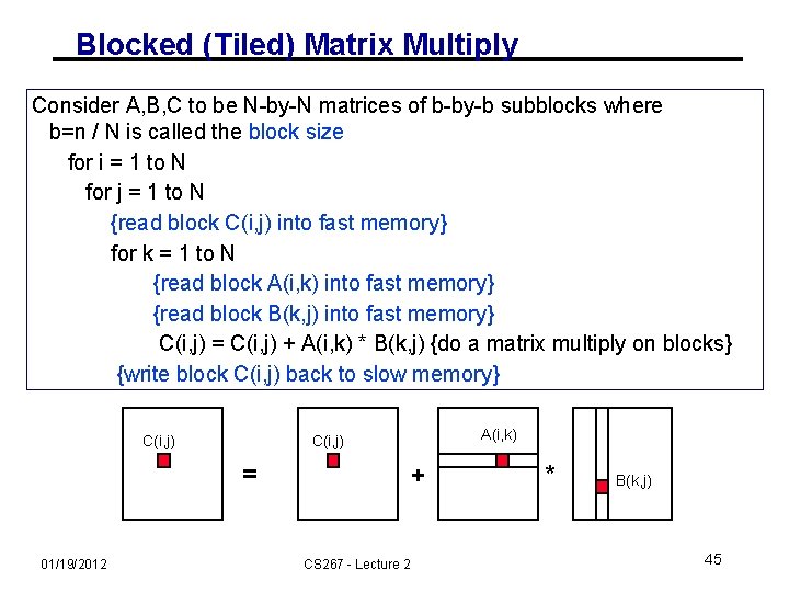
Blocked (Tiled) Matrix Multiply Consider A, B, C to be N-by-N matrices of b-by-b subblocks where b=n / N is called the block size for i = 1 to N for j = 1 to N {read block C(i, j) into fast memory} for k = 1 to N {read block A(i, k) into fast memory} {read block B(k, j) into fast memory} C(i, j) = C(i, j) + A(i, k) * B(k, j) {do a matrix multiply on blocks} {write block C(i, j) back to slow memory} C(i, j) = 01/19/2012 A(i, k) C(i, j) + CS 267 - Lecture 2 * B(k, j) 45

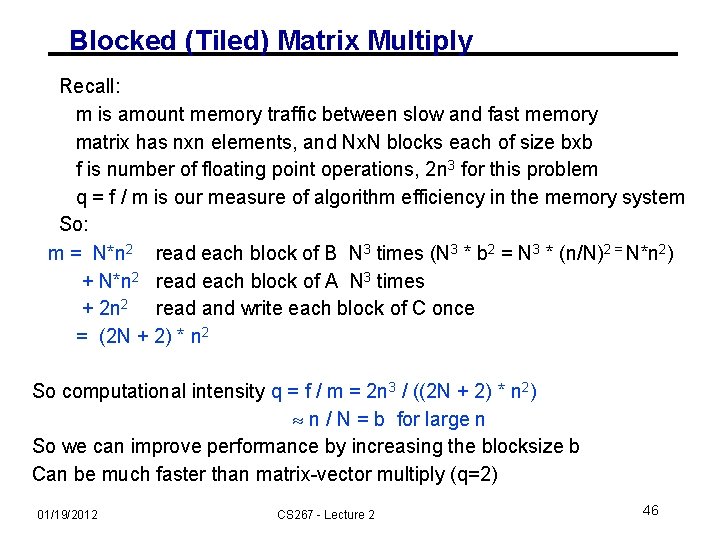
Blocked (Tiled) Matrix Multiply Recall: m is amount memory traffic between slow and fast memory matrix has nxn elements, and Nx. N blocks each of size bxb f is number of floating point operations, 2 n 3 for this problem q = f / m is our measure of algorithm efficiency in the memory system So: m = N*n 2 read each block of B N 3 times (N 3 * b 2 = N 3 * (n/N)2 = N*n 2) + N*n 2 read each block of A N 3 times + 2 n 2 read and write each block of C once = (2 N + 2) * n 2 So computational intensity q = f / m = 2 n 3 / ((2 N + 2) * n 2) n / N = b for large n So we can improve performance by increasing the blocksize b Can be much faster than matrix-vector multiply (q=2) 01/19/2012 CS 267 - Lecture 2 46

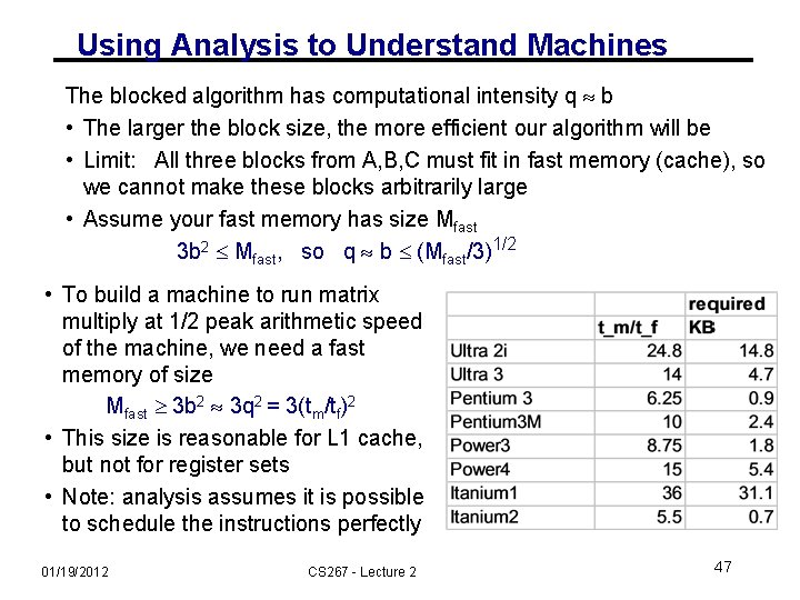
Using Analysis to Understand Machines The blocked algorithm has computational intensity q b • The larger the block size, the more efficient our algorithm will be • Limit: All three blocks from A, B, C must fit in fast memory (cache), so we cannot make these blocks arbitrarily large • Assume your fast memory has size Mfast 3 b 2 Mfast, so q b (Mfast/3)1/2 • To build a machine to run matrix multiply at 1/2 peak arithmetic speed of the machine, we need a fast memory of size Mfast 3 b 2 3 q 2 = 3(tm/tf)2 • This size is reasonable for L 1 cache, but not for register sets • Note: analysis assumes it is possible to schedule the instructions perfectly 01/19/2012 CS 267 - Lecture 2 47

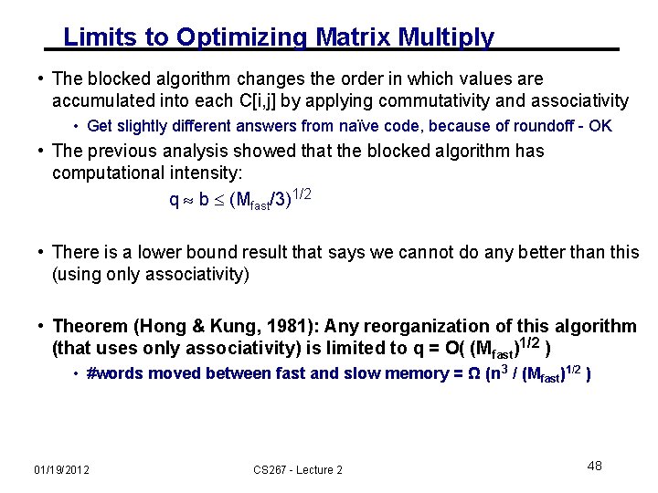
Limits to Optimizing Matrix Multiply • The blocked algorithm changes the order in which values are accumulated into each C[i, j] by applying commutativity and associativity • Get slightly different answers from naïve code, because of roundoff - OK • The previous analysis showed that the blocked algorithm has computational intensity: q b (Mfast/3)1/2 • There is a lower bound result that says we cannot do any better than this (using only associativity) • Theorem (Hong & Kung, 1981): Any reorganization of this algorithm (that uses only associativity) is limited to q = O( (Mfast)1/2 ) • #words moved between fast and slow memory = Ω (n 3 / (Mfast)1/2 ) 01/19/2012 CS 267 - Lecture 2 48

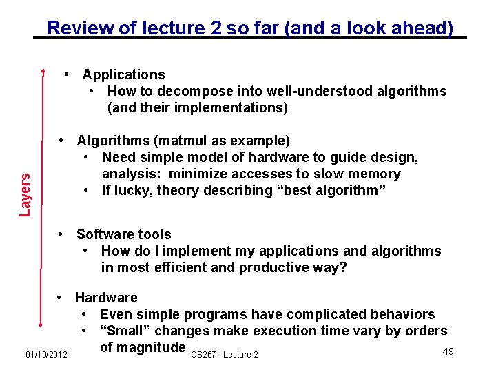
Review of lecture 2 so far (and a look ahead) Layers • Applications • How to decompose into well-understood algorithms (and their implementations) • Algorithms (matmul as example) • Need simple model of hardware to guide design, analysis: minimize accesses to slow memory • If lucky, theory describing “best algorithm” • Software tools • How do I implement my applications and algorithms in most efficient and productive way? • Hardware • Even simple programs have complicated behaviors • “Small” changes make execution time vary by orders of magnitude CS 267 - Lecture 2 49 01/19/2012

Communication lower bounds for Matmul • Hong/Kung theorem is a lower bound on amount of data communicated by matmul • Number of words moved between fast and slow memory (cache and DRAM, or DRAM and disk, or …) = Ω (n 3 / Mfast 1/2) • Cost of moving data may also depend on the number of “messages” into which data is packed • Eg: number of cache lines, disk accesses, … • #messages = Ω (n 3 / Mfast 3/2) • Lower bounds extend to anything “similar enough” to 3 nested loops • Rest of linear algebra (solving linear systems, least squares…) • Dense and sparse matrices • Sequential and parallel algorithms, … • Need (more) new algorithms to attain these lower bounds… 01/19/2012 CS 267 - Lecture 2 50

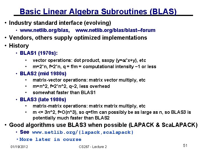
Basic Linear Algebra Subroutines (BLAS) • Industry standard interface (evolving) • www. netlib. org/blas, www. netlib. org/blast--forum • Vendors, others supply optimized implementations • History • BLAS 1 (1970 s): • • vector operations: dot product, saxpy (y=a*x+y), etc m=2*n, f=2*n, q = f/m = computational intensity ~1 or less • BLAS 2 (mid 1980 s) • • • matrix-vector operations: matrix vector multiply, etc m=n^2, f=2*n^2, q~2, less overhead somewhat faster than BLAS 1 • BLAS 3 (late 1980 s) • • matrix-matrix operations: matrix multiply, etc m <= 3 n^2, f=O(n^3), so q=f/m can possibly be as large as n, so BLAS 3 is potentially much faster than BLAS 2 • Good algorithms use BLAS 3 when possible (LAPACK & Sca. LAPACK) • See www. netlib. org/{lapack, scalapack} • More later in course 01/19/2012 CS 267 - Lecture 2 51

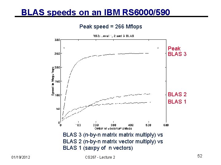
BLAS speeds on an IBM RS 6000/590 Peak speed = 266 Mflops Peak BLAS 3 BLAS 2 BLAS 1 BLAS 3 (n-by-n matrix multiply) vs BLAS 2 (n-by-n matrix vector multiply) vs BLAS 1 (saxpy of n vectors) 01/19/2012 CS 267 - Lecture 2 52

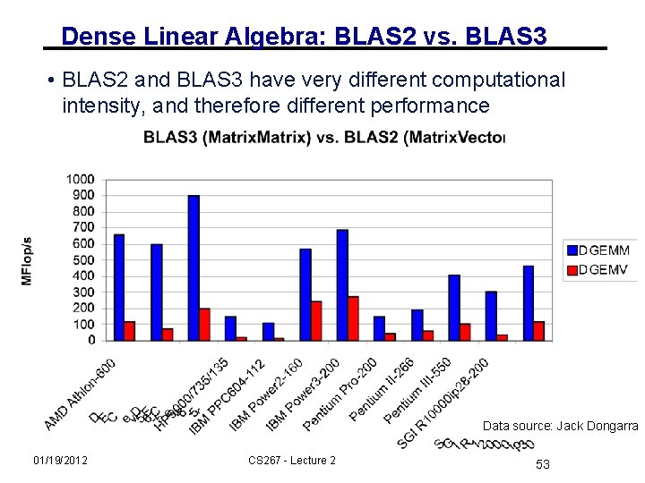
Dense Linear Algebra: BLAS 2 vs. BLAS 3 • BLAS 2 and BLAS 3 have very different computational intensity, and therefore different performance Data source: Jack Dongarra 01/19/2012 CS 267 - Lecture 2 53

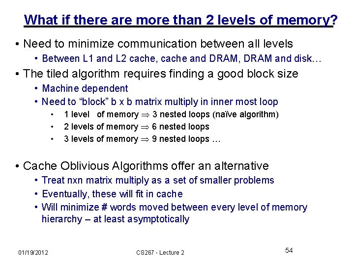
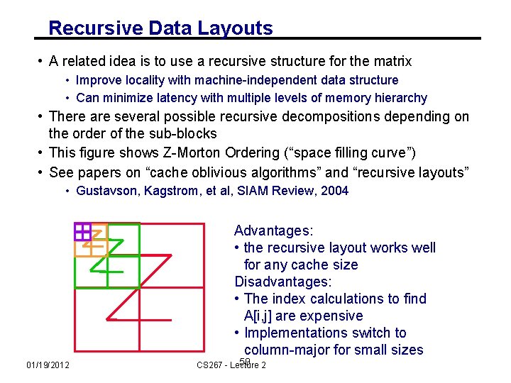
What if there are more than 2 levels of memory? • Need to minimize communication between all levels • Between L 1 and L 2 cache, cache and DRAM, DRAM and disk… • The tiled algorithm requires finding a good block size • Machine dependent • Need to “block” b x b matrix multiply in inner most loop • • • 1 level of memory 3 nested loops (naïve algorithm) 2 levels of memory 6 nested loops 3 levels of memory 9 nested loops … • Cache Oblivious Algorithms offer an alternative • Treat nxn matrix multiply as a set of smaller problems • Eventually, these will fit in cache • Will minimize # words moved between every level of memory hierarchy – at least asymptotically 01/19/2012 CS 267 - Lecture 2 54

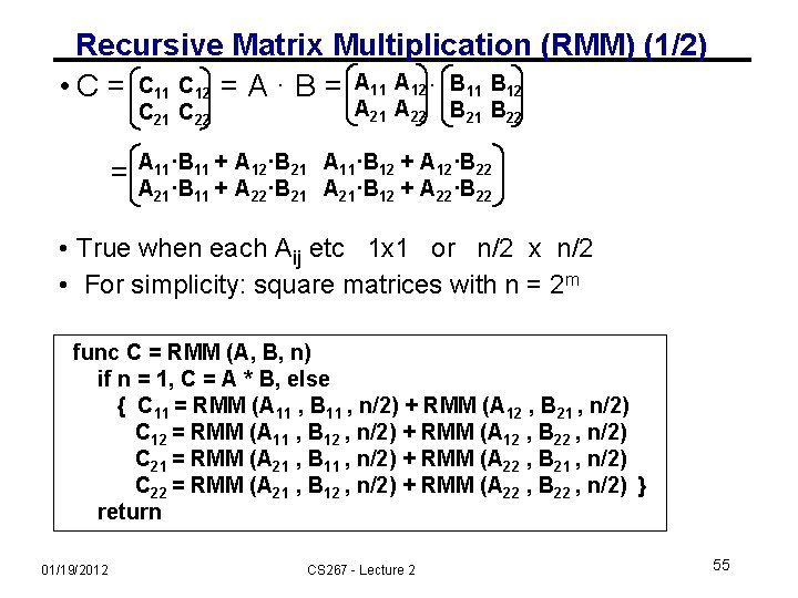
Recursive Matrix Multiplication (RMM) (1/2) • C = C 11 C 12 = A · B = A 11 A 12 · B 11 B 12 C 21 C 22 = A 21 A 22 B 21 B 22 A 11·B 11 + A 12·B 21 A 11·B 12 + A 12·B 22 A 21·B 11 + A 22·B 21 A 21·B 12 + A 22·B 22 • True when each Aij etc 1 x 1 or n/2 x n/2 • For simplicity: square matrices with n = 2 m func C = RMM (A, B, n) if n = 1, C = A * B, else { C 11 = RMM (A 11 , B 11 , n/2) + RMM (A 12 , B 21 , n/2) C 12 = RMM (A 11 , B 12 , n/2) + RMM (A 12 , B 22 , n/2) C 21 = RMM (A 21 , B 11 , n/2) + RMM (A 22 , B 21 , n/2) C 22 = RMM (A 21 , B 12 , n/2) + RMM (A 22 , B 22 , n/2) } return 01/19/2012 CS 267 - Lecture 2 55

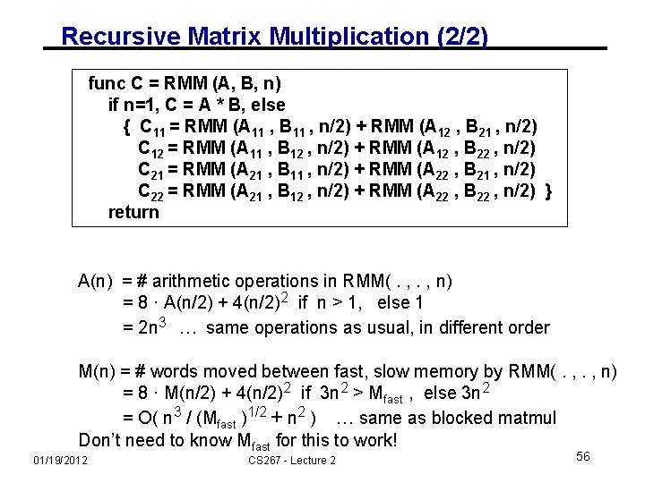
Recursive Matrix Multiplication (2/2) func C = RMM (A, B, n) if n=1, C = A * B, else { C 11 = RMM (A 11 , B 11 , n/2) + RMM (A 12 , B 21 , n/2) C 12 = RMM (A 11 , B 12 , n/2) + RMM (A 12 , B 22 , n/2) C 21 = RMM (A 21 , B 11 , n/2) + RMM (A 22 , B 21 , n/2) C 22 = RMM (A 21 , B 12 , n/2) + RMM (A 22 , B 22 , n/2) } return A(n) = # arithmetic operations in RMM(. , n) = 8 · A(n/2) + 4(n/2)2 if n > 1, else 1 = 2 n 3 … same operations as usual, in different order M(n) = # words moved between fast, slow memory by RMM(. , n) = 8 · M(n/2) + 4(n/2)2 if 3 n 2 > Mfast , else 3 n 2 = O( n 3 / (Mfast )1/2 + n 2 ) … same as blocked matmul Don’t need to know Mfast for this to work! 01/19/2012 CS 267 - Lecture 2 56

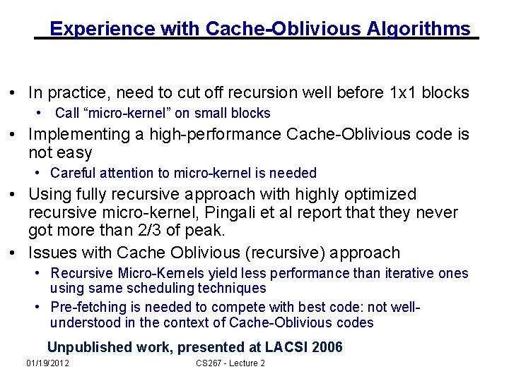
Experience with Cache-Oblivious Algorithms • In practice, need to cut off recursion well before 1 x 1 blocks • Call “micro-kernel” on small blocks • Implementing a high-performance Cache-Oblivious code is not easy • Careful attention to micro-kernel is needed • Using fully recursive approach with highly optimized recursive micro-kernel, Pingali et al report that they never got more than 2/3 of peak. • Issues with Cache Oblivious (recursive) approach • Recursive Micro-Kernels yield less performance than iterative ones using same scheduling techniques • Pre-fetching is needed to compete with best code: not wellunderstood in the context of Cache-Oblivious codes Unpublished work, presented at LACSI 2006 01/19/2012 CS 267 - Lecture 2

Recursive Data Layouts • A related idea is to use a recursive structure for the matrix • Improve locality with machine-independent data structure • Can minimize latency with multiple levels of memory hierarchy • There are several possible recursive decompositions depending on the order of the sub-blocks • This figure shows Z-Morton Ordering (“space filling curve”) • See papers on “cache oblivious algorithms” and “recursive layouts” • Gustavson, Kagstrom, et al, SIAM Review, 2004 Advantages: • the recursive layout works well for any cache size Disadvantages: • The index calculations to find A[i, j] are expensive • Implementations switch to column-major for small sizes 01/19/2012 59 2 CS 267 - Lecture

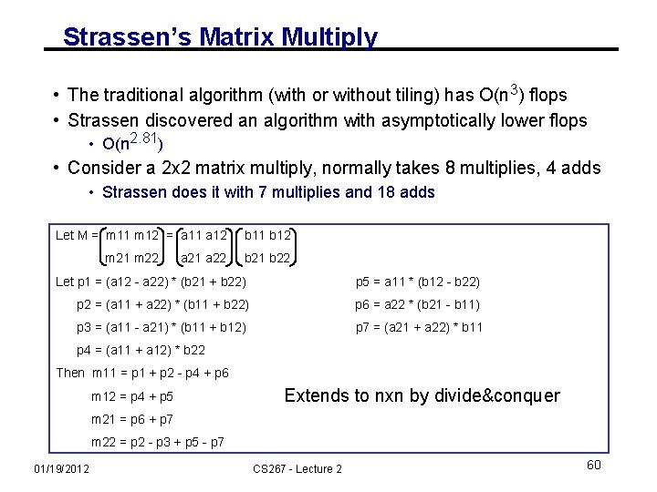
Strassen’s Matrix Multiply • The traditional algorithm (with or without tiling) has O(n 3) flops • Strassen discovered an algorithm with asymptotically lower flops • O(n 2. 81) • Consider a 2 x 2 matrix multiply, normally takes 8 multiplies, 4 adds • Strassen does it with 7 multiplies and 18 adds Let M = m 11 m 12 = a 11 a 12 b 11 b 12 m 21 m 22 = a 21 a 22 b 21 b 22 Let p 1 = (a 12 - a 22) * (b 21 + b 22) p 5 = a 11 * (b 12 - b 22) p 2 = (a 11 + a 22) * (b 11 + b 22) p 6 = a 22 * (b 21 - b 11) p 3 = (a 11 - a 21) * (b 11 + b 12) p 7 = (a 21 + a 22) * b 11 p 4 = (a 11 + a 12) * b 22 Then m 11 = p 1 + p 2 - p 4 + p 6 m 12 = p 4 + p 5 Extends to nxn by divide&conquer m 21 = p 6 + p 7 m 22 = p 2 - p 3 + p 5 - p 7 01/19/2012 CS 267 - Lecture 2 60

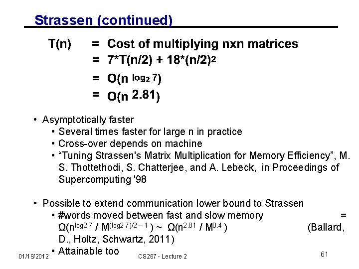
Strassen (continued) • Asymptotically faster • Several times faster for large n in practice • Cross-over depends on machine • “Tuning Strassen's Matrix Multiplication for Memory Efficiency”, M. S. Thottethodi, S. Chatterjee, and A. Lebeck, in Proceedings of Supercomputing '98 • Possible to extend communication lower bound to Strassen • #words moved between fast and slow memory = Ω(nlog 2 7 / M(log 2 7)/2 – 1 ) ~ Ω(n 2. 81 / M 0. 4 ) (Ballard, D. , Holtz, Schwartz, 2011) • Attainable too 61 01/19/2012 CS 267 - Lecture 2

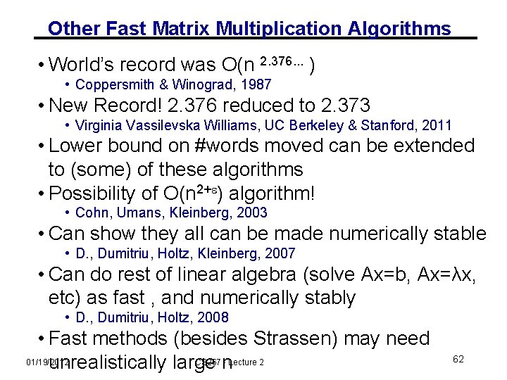
Other Fast Matrix Multiplication Algorithms • World’s record was O(n 2. 376. . . ) • Coppersmith & Winograd, 1987 • New Record! 2. 376 reduced to 2. 373 • Virginia Vassilevska Williams, UC Berkeley & Stanford, 2011 • Lower bound on #words moved can be extended to (some) of these algorithms • Possibility of O(n 2+ ) algorithm! • Cohn, Umans, Kleinberg, 2003 • Can show they all can be made numerically stable • D. , Dumitriu, Holtz, Kleinberg, 2007 • Can do rest of linear algebra (solve Ax=b, Ax=λx, etc) as fast , and numerically stably • D. , Dumitriu, Holtz, 2008 • Fast methods (besides Strassen) may need 01/19/2012 CS 267 n - Lecture 2 unrealistically large 62

Tuning Code in Practice • Tuning code can be tedious • Lots of code variations to try besides blocking • Machine hardware performance hard to predict • Compiler behavior hard to predict • Response: “Autotuning” • Let computer generate large set of possible code variations, and search them for the fastest ones • Field started with CS 267 homework assignment in mid 1990 s • • PHi. PAC, leading to ATLAS, incorporated in Matlab We still use the same assignment • We (and others) are extending autotuning to other dwarfs / motifs • Still need to understand how to do it by hand • Not every code will have an autotuner • Need to know if you want to build autotuners 01/19/2012 CS 267 - Lecture 2 63

Search Over Block Sizes • Performance models are useful for high level algorithms • Helps in developing a blocked algorithm • Models have not proven very useful for block size selection • too complicated to be useful – See work by Sid Chatterjee for detailed model • too simple to be accurate – Multiple multidimensional arrays, virtual memory, etc. • Speed depends on matrix dimensions, details of code, compiler, processor 01/19/2012 CS 267 - Lecture 2 64

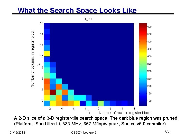
Number of columns in register block What the Search Space Looks Like Number of rows in register block A 2 -D slice of a 3 -D register-tile search space. The dark blue region was pruned. (Platform: Sun Ultra-IIi, 333 MHz, 667 Mflop/s peak, Sun cc v 5. 0 compiler) 01/19/2012 CS 267 - Lecture 2 65

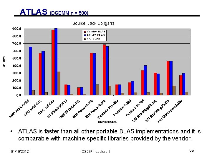
ATLAS (DGEMM n = 500) Source: Jack Dongarra • ATLAS is faster than all other portable BLAS implementations and it is comparable with machine-specific libraries provided by the vendor. 01/19/2012 CS 267 - Lecture 2 66

Optimizing in Practice • Tiling for registers • loop unrolling, use of named “register” variables • Tiling for multiple levels of cache and TLB • Exploiting fine-grained parallelism in processor • superscalar; pipelining • Complicated compiler interactions • Hard to do by hand (but you’ll try) • Automatic optimization an active research area • Par. Lab: parlab. eecs. berkeley. edu • Be. BOP: bebop. cs. berkeley. edu • Weekly group meeting Tuesdays 12: 30 pm • PHi. PAC: www. icsi. berkeley. edu/~bilmes/phipac in particular tr-98 -035. ps. gz • ATLAS: www. netlib. org/atlas 01/19/2012 CS 267 - Lecture 2 67

Removing False Dependencies • Using local variables, reorder operations to remove false dependencies a[i] = b[i] + c; a[i+1] = b[i+1] * d; false read-after-write hazard between a[i] and b[i+1] float f 1 = b[i]; float f 2 = b[i+1]; a[i] = f 1 + c; a[i+1] = f 2 * d; With some compilers, you can declare a and b unaliased. • Done via “restrict pointers, ” compiler flag, or pragma) 01/19/2012 CS 267 - Lecture 2 68

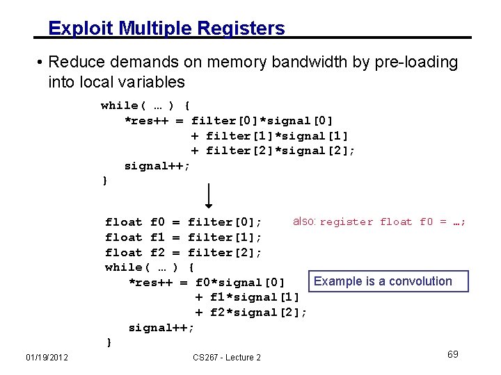
Exploit Multiple Registers • Reduce demands on memory bandwidth by pre-loading into local variables while( … ) { *res++ = filter[0]*signal[0] + filter[1]*signal[1] + filter[2]*signal[2]; signal++; } also: register float f 0 = …; float f 0 = filter[0]; float f 1 = filter[1]; float f 2 = filter[2]; while( … ) { Example is a convolution *res++ = f 0*signal[0] + f 1*signal[1] + f 2*signal[2]; signal++; } 01/19/2012 CS 267 - Lecture 2 69

Loop Unrolling • Expose instruction-level parallelism float f 0 = filter[0], f 1 = filter[1], f 2 = filter[2]; float s 0 = signal[0], s 1 = signal[1], s 2 = signal[2]; *res++ = f 0*s 0 + f 1*s 1 + f 2*s 2; do { signal += 3; s 0 = signal[0]; res[0] = f 0*s 1 + f 1*s 2 + f 2*s 0; s 1 = signal[1]; res[1] = f 0*s 2 + f 1*s 0 + f 2*s 1; s 2 = signal[2]; res[2] = f 0*s 0 + f 1*s 1 + f 2*s 2; res += 3; } while( … ); 01/19/2012 CS 267 - Lecture 2 70

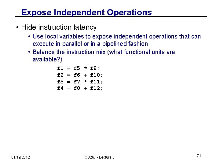
Expose Independent Operations • Hide instruction latency • Use local variables to expose independent operations that can execute in parallel or in a pipelined fashion • Balance the instruction mix (what functional units are available? ) f 1 f 2 f 3 f 4 01/19/2012 = = f 5 f 6 f 7 f 8 * + f 9; f 10; f 11; f 12; CS 267 - Lecture 2 71

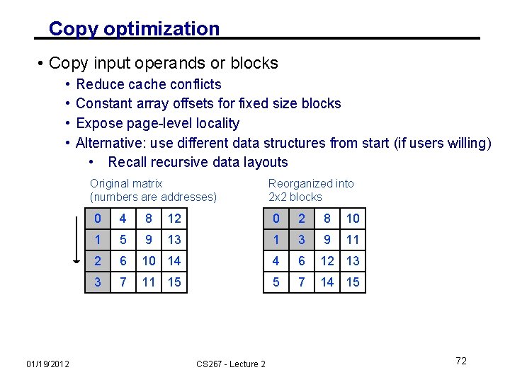
Copy optimization • Copy input operands or blocks • • Reduce cache conflicts Constant array offsets for fixed size blocks Expose page-level locality Alternative: use different data structures from start (if users willing) • Recall recursive data layouts Original matrix (numbers are addresses) 01/19/2012 Reorganized into 2 x 2 blocks 0 4 8 12 0 2 8 10 1 5 9 13 1 3 9 11 2 6 10 14 4 6 12 13 3 7 11 15 5 7 14 15 CS 267 - Lecture 2 72

Locality in Other Algorithms • The performance of any algorithm is limited by q • q = “computational intensity” = #arithmetic_ops / #words_moved • In matrix multiply, we increase q by changing computation order • increased temporal locality • For other algorithms and data structures, even handtransformations are still an open problem • Lots of open problems, class projects 01/19/2012 CS 267 - Lecture 2 73

Summary of Lecture 2 • Details of machine are important for performance • Processor and memory system (not just parallelism) • Before you parallelize, make sure you’re getting good serial performance • What to expect? Use understanding of hardware limits • There is parallelism hidden within processors • Pipelining, SIMD, etc • Machines have memory hierarchies • 100 s of cycles to read from DRAM (main memory) • Caches are fast (small) memory that optimize average case • Locality is at least as important as computation • Temporal: re-use of data recently used • Spatial: using data nearby that recently used • Can rearrange code/data to improve locality • Goal: minimize communication = data movement 01/19/2012 CS 267 - Lecture 2 74

Class Logistics • Homework 0 posted on web site • Find and describe interesting application of parallelism • Due Feb 2 • Could even be your intended class project • Homework 1 posted on web site • Tuning matrix multiply • Due Feb 14 • Please fill in on-line class survey • We need this to assign teams for Homework 1 01/19/2012 CS 267 - Lecture 2 75

Some reading for today (see website) • Sourcebook Chapter 3, (note that chapters 2 and 3 cover the material of lecture 2 and lecture 3, but not in the same order). • "Performance Optimization of Numerically Intensive Codes", by Stefan Goedecker and Adolfy Hoisie, SIAM 2001. • Web pages for reference: • Be. BOP Homepage • ATLAS Homepage • BLAS (Basic Linear Algebra Subroutines), Reference for (unoptimized) implementations of the BLAS, with documentation. • LAPACK (Linear Algebra PACKage), a standard linear algebra library optimized to use the BLAS effectively on uniprocessors and shared memory machines (software, documentation and reports) • Sca. LAPACK (Scalable LAPACK), a parallel version of LAPACK for distributed memory machines (software, documentation and reports) • Tuning Strassen's Matrix Multiplication for Memory Efficiency Mithuna S. Thottethodi, Siddhartha Chatterjee, and Alvin R. Lebeck in Proceedings of Supercomputing '98, November 1998 postscript • Recursive Array Layouts and Fast Parallel Matrix Multiplication” by Chatterjee et al. IEEE TPDS November 2002. 01/19/2012 CS 267 - Lecture 2 76

Extra Slides 01/19/2012 CS 267 - Lecture 2 77