Indexing Implementation and Indexing Models CSC 575 Intelligent

Indexing Implementation and Indexing Models CSC 575 Intelligent Information Retrieval

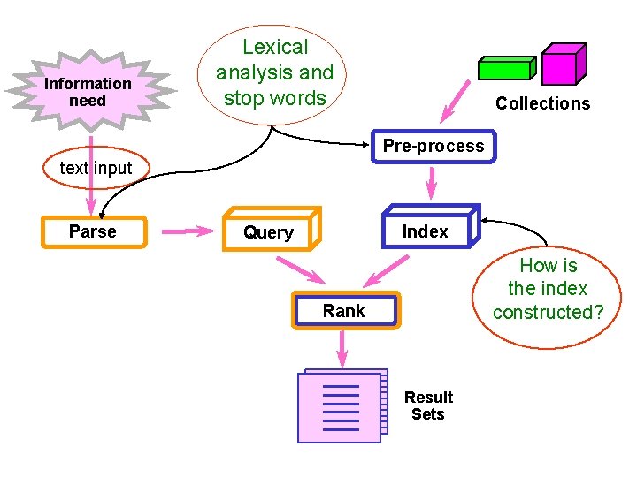
Information need Lexical analysis and stop words Collections Pre-process text input Parse Index Query How is the index constructed? Rank Result Sets

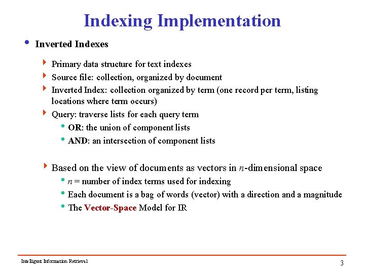
Indexing Implementation i Inverted Indexes 4 Primary data structure for text indexes 4 Source file: collection, organized by document 4 Inverted Index: collection organized by term (one record per term, listing locations where term occurs) 4 Query: traverse lists for each query term i. OR: the union of component lists i. AND: an intersection of component lists 4 Based on the view of documents as vectors in n-dimensional space in = number of index terms used for indexing i. Each document is a bag of words (vector) with a direction and a magnitude i. The Vector-Space Model for IR Intelligent Information Retrieval 3

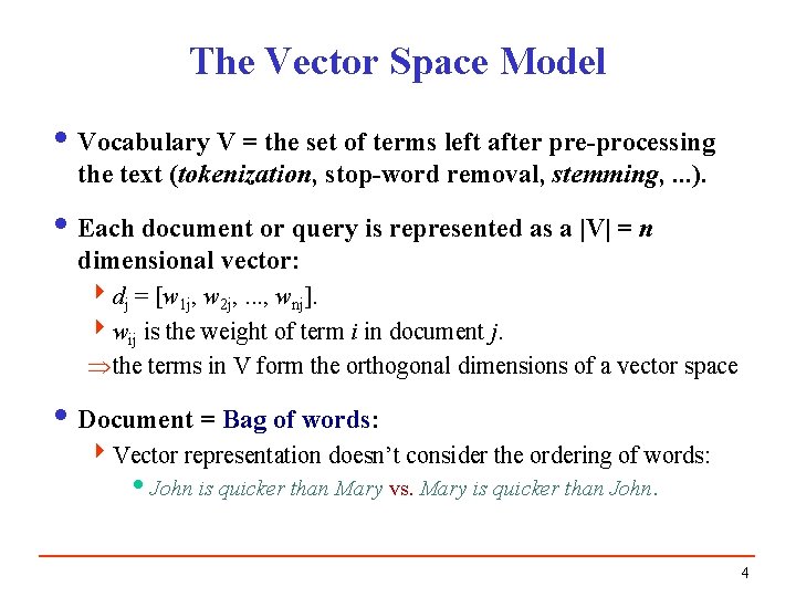
The Vector Space Model i Vocabulary V = the set of terms left after pre-processing the text (tokenization, stop-word removal, stemming, . . . ). i Each document or query is represented as a |V| = n dimensional vector: 4 dj = [w 1 j, w 2 j, . . . , wnj]. 4 wij is the weight of term i in document j. the terms in V form the orthogonal dimensions of a vector space i Document = Bag of words: 4 Vector representation doesn’t consider the ordering of words: i. John is quicker than Mary vs. Mary is quicker than John. 4

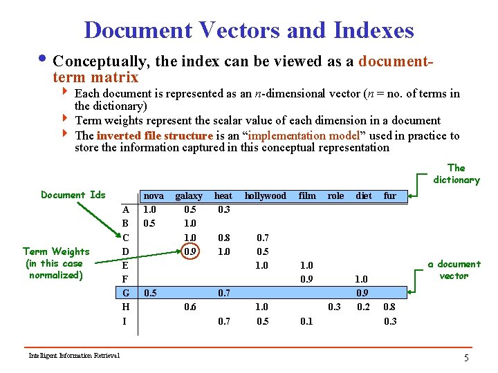
Document Vectors and Indexes i Conceptually, the index can be viewed as a documentterm matrix 4 Each document is represented as an n-dimensional vector (n = no. of terms in the dictionary) 4 Term weights represent the scalar value of each dimension in a document 4 The inverted file structure is an “implementation model” used in practice to store the information captured in this conceptual representation The dictionary Document Ids Term Weights (in this case normalized) Intelligent Information Retrieval A B C D E F G H I nova 1. 0 0. 5 galaxy 0. 5 1. 0 0. 9 0. 5 heat 0. 3 0. 8 1. 0 hollywood 0. 7 0. 5 1. 0 film role 1. 0 0. 9 0. 7 0. 6 0. 7 1. 0 0. 5 0. 3 0. 1 diet 1. 0 0. 9 0. 2 fur a document vector 0. 8 0. 3 5

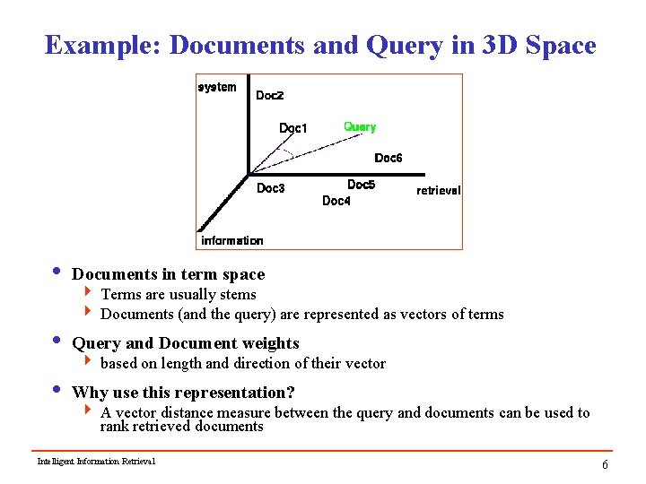
Example: Documents and Query in 3 D Space i Documents in term space 4 Terms are usually stems 4 Documents (and the query) are represented as vectors of terms i Query and Document weights 4 based on length and direction of their vector i Why use this representation? 4 A vector distance measure between the query and documents can be used to rank retrieved documents Intelligent Information Retrieval 6

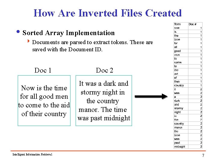
How Are Inverted Files Created i Sorted Array Implementation 4 Documents are parsed to extract tokens. These are saved with the Document ID. Doc 1 Doc 2 Now is the time for all good men to come to the aid of their country It was a dark and stormy night in the country manor. The time was past midnight Intelligent Information Retrieval 7

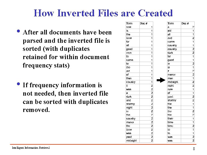
How Inverted Files are Created i After all documents have been parsed and the inverted file is sorted (with duplicates retained for within document frequency stats) i If frequency information is not needed, then inverted file can be sorted with duplicates removed. Intelligent Information Retrieval 8

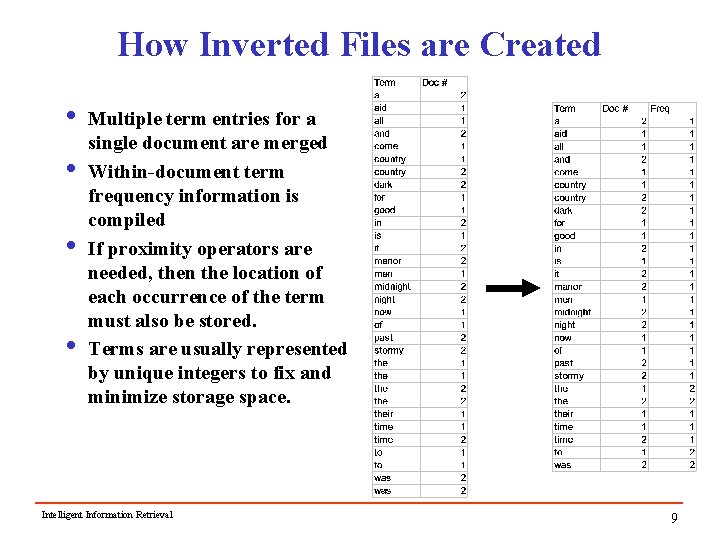
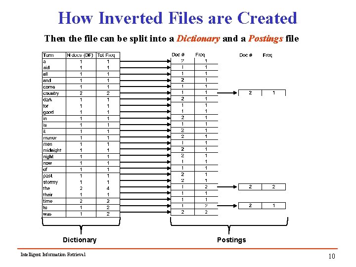
How Inverted Files are Created i Multiple term entries for a single document are merged i Within-document term frequency information is compiled i If proximity operators are needed, then the location of each occurrence of the term must also be stored. i Terms are usually represented by unique integers to fix and minimize storage space. Intelligent Information Retrieval 9

How Inverted Files are Created Then the file can be split into a Dictionary and a Postings file Dictionary Intelligent Information Retrieval Postings 10

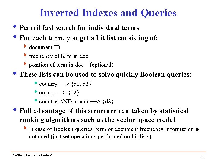
Inverted Indexes and Queries i Permit fast search for individual terms i For each term, you get a hit list consisting of: 4 document ID 4 frequency of term in doc 4 position of term in doc (optional) i These lists can be used to solve quickly Boolean queries: icountry ==> {d 1, d 2} imanor ==> {d 2} icountry AND manor ==> {d 2} i Full advantage of this structure can taken by statistical ranking algorithms such as the vector space model 4 in case of Boolean queries, term or document frequency information is not used (just set operations performed on hit lists) Intelligent Information Retrieval 11

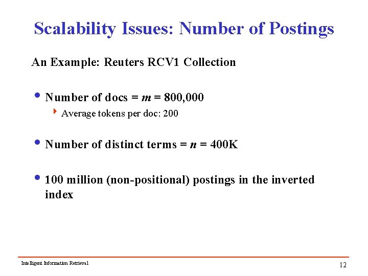
Scalability Issues: Number of Postings An Example: Reuters RCV 1 Collection i Number of docs = m = 800, 000 4 Average tokens per doc: 200 i Number of distinct terms = n = 400 K i 100 million (non-positional) postings in the inverted index Intelligent Information Retrieval 12

Bottleneck i Parse and build postings entries one doc at a time i Sort postings entries by term (then by doc within each term) i Doing this with random disk seeks would be too slow – must sort N=100 M records If every comparison took 2 disk seeks (10 milliseconds each), and N items could be sorted with N log 2 N comparisons, how long would this take? Intelligent Information Retrieval 13

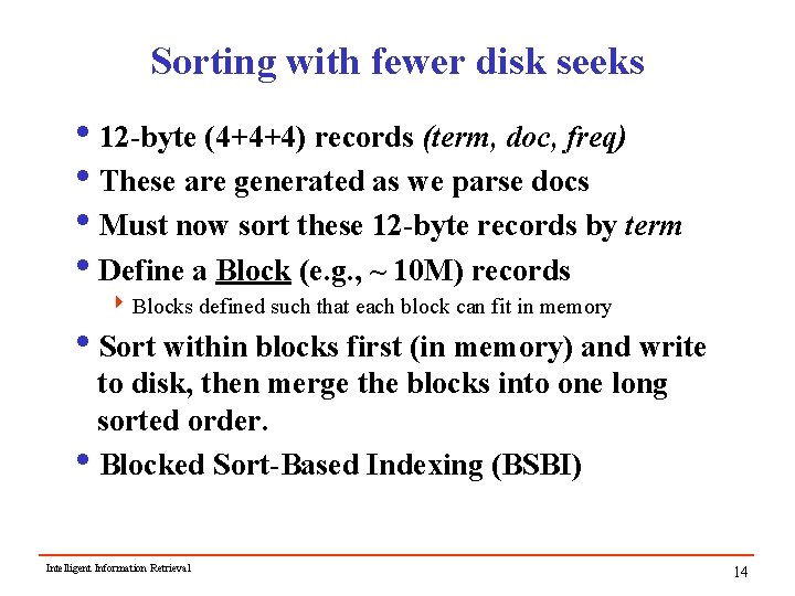
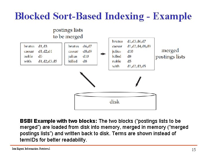
Sorting with fewer disk seeks i 12 -byte (4+4+4) records (term, doc, freq) i. These are generated as we parse docs i. Must now sort these 12 -byte records by term i. Define a Block (e. g. , ~ 10 M) records 4 Blocks defined such that each block can fit in memory i. Sort within blocks first (in memory) and write to disk, then merge the blocks into one long sorted order. i. Blocked Sort-Based Indexing (BSBI) Intelligent Information Retrieval 14

Blocked Sort-Based Indexing - Example BSBI Example with two blocks: The two blocks (“postings lists to be merged”) are loaded from disk into memory, merged in memory (“merged postings lists”) and written back to disk. Terms are shown instead of term. IDs for better readability. Intelligent Information Retrieval 15

Sec. 4. 3 Problem with Sort-Based Algorithm i Assumption: we can keep the dictionary in memory. i We need the dictionary (which grows dynamically) in order to implement a term to term. ID mapping. i Actually, we could work with term, doc. ID postings instead of term. ID, doc. ID postings. . . i. . . but then intermediate files become very large. (We would end up with a scalable, but very slow index construction method. )

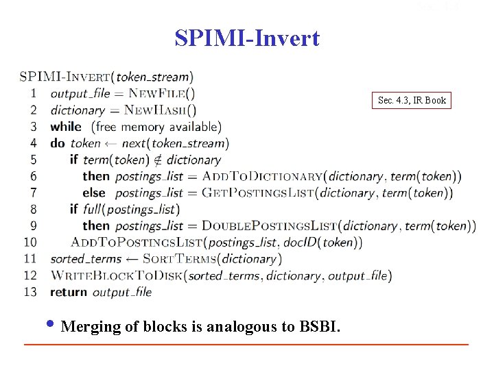
Sec. 4. 3 SPIMI: Single-pass in-memory indexing i Key idea 1: Generate separate dictionaries for each block – no need to maintain term-term. ID mapping across blocks. i Key idea 2: Don’t sort. Accumulate postings in postings lists as they occur. i With these two ideas we can generate a complete inverted index for each block. i These separate indexes can then be merged into one big index.

Sec. 4. 3 SPIMI-Invert Sec. 4. 3, IR Book i Merging of blocks is analogous to BSBI.

Distributed indexing i For web-scale indexing 4 must use a distributed computing cluster i Individual machines are fault-prone 4 Can unpredictably slow down or fail i How do we exploit such a pool of machines? 4 Maintain a master machine directing the indexing job – considered “safe”. 4 Break up indexing into sets of (parallel) tasks. 4 Master machine assigns each task to an idle machine from a pool. Intelligent Information Retrieval 19

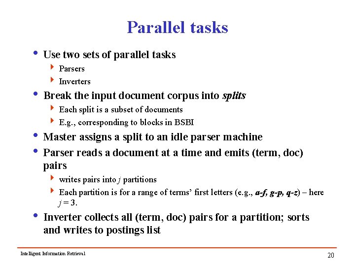
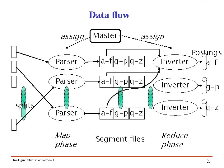
Parallel tasks i Use two sets of parallel tasks 4 Parsers 4 Inverters i Break the input document corpus into splits 4 Each split is a subset of documents 4 E. g. , corresponding to blocks in BSBI i Master assigns a split to an idle parser machine i Parser reads a document at a time and emits (term, doc) pairs 4 writes pairs into j partitions 4 Each partition is for a range of terms’ first letters (e. g. , a-f, g-p, q-z) – here j = 3. i Inverter collects all (term, doc) pairs for a partition; sorts and writes to postings list Intelligent Information Retrieval 20

Sec. 4. 4 Data flow assign splits Intelligent Information Retrieval Master assign Parser a-f g-p q-z Map phase Segment files Postings Inverter a-f Inverter g-p Inverter q-z Reduce phase 21

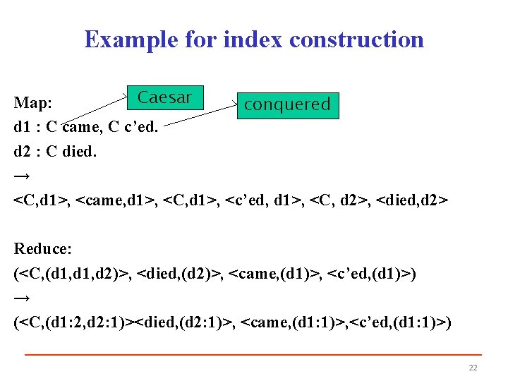
Example for index construction Caesar Map: conquered d 1 : C came, C c’ed. d 2 : C died. → <C, d 1>, <came, d 1>, <C, d 1>, <c’ed, d 1>, <C, d 2>, <died, d 2> Reduce: (<C, (d 1, d 2)>, <died, (d 2)>, <came, (d 1)>, <c’ed, (d 1)>) → (<C, (d 1: 2, d 2: 1)><died, (d 2: 1)>, <came, (d 1: 1)>, <c’ed, (d 1: 1)>) 22

Dynamic indexing i. Problem: 4 Docs come in over time ipostings updates for terms already in dictionary inew terms added to dictionary 4 Docs get deleted i Simplest Approach 4 Maintain a “big” main index 4 New docs go into a “small” auxiliary index 4 Search across both, merge results 4 Deletions i. Invalidation bit-vector for deleted docs i. Filter docs output on a search result by this invalidation bit-vector 4 Periodically, re-index into one main index Intelligent Information Retrieval 23

Index on disk vs. memory i. Most retrieval systems keep the dictionary in memory and the postings on disk i. Web search engines frequently keep both in memory 4 massive memory requirement 4 feasible for large web service installations 4 less so for commercial usage where query loads are lighter Intelligent Information Retrieval 24

Retrieval From Indexes i Given the large indexes in IR applications, searching for keys in the dictionaries becomes a dominant cost i Two main choices for dictionary data structures: Hashtables or Trees 4 Using Hashing irequires the derivation of a hash function mapping terms to locations imay require collision detection and resolution for non-unique hash values 4 Using Trees i. Binary search trees inice properties, easy to implement, and effective ienhancements such as B+ trees can improve search effectiveness ibut, requires the storage of keys in each internal node Intelligent Information Retrieval 25

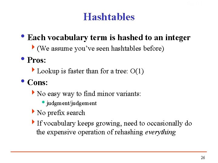
Sec. 3. 1 Hashtables i. Each vocabulary term is hashed to an integer 4(We assume you’ve seen hashtables before) i. Pros: 4 Lookup is faster than for a tree: O(1) i. Cons: 4 No easy way to find minor variants: ijudgment/judgement 4 No prefix search 4 If vocabulary keeps growing, need to occasionally do the expensive operation of rehashing everything 26

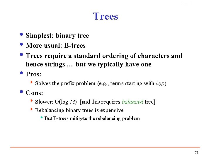
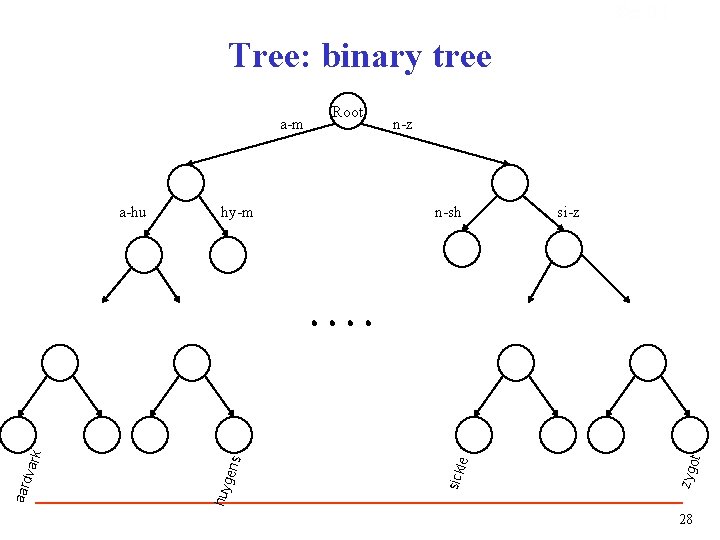
Sec. 3. 1 Trees i Simplest: binary tree i More usual: B-trees i Trees require a standard ordering of characters and hence strings … but we typically have one i Pros: 4 Solves the prefix problem (e. g. , terms starting with hyp) i Cons: 4 Slower: O(log M) [and this requires balanced tree] 4 Rebalancing binary trees is expensive i. But B-trees mitigate the rebalancing problem 27

Sec. 3. 1 Tree: binary tree n-z si-z ot n-sh zyg gen s hy-m huy aard vark a-hu Root sick le a-m 28

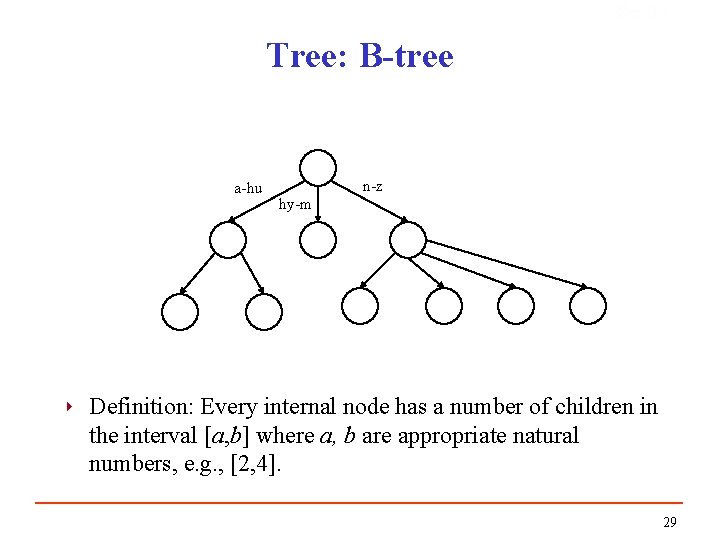
Sec. 3. 1 Tree: B-tree a-hu 4 n-z hy-m Definition: Every internal node has a number of children in the interval [a, b] where a, b are appropriate natural numbers, e. g. , [2, 4]. 29

Recall: Steps in Basic Automatic Indexing i Parse documents to recognize structure i Scan for word tokens i Stopword removal i Stem words i Weight words Intelligent Information Retrieval 30

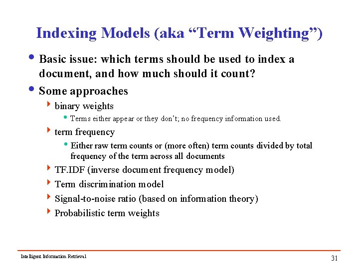
Indexing Models (aka “Term Weighting”) i Basic issue: which terms should be used to index a document, and how much should it count? i Some approaches 4 binary weights i Terms either appear or they don’t; no frequency information used. 4 term frequency i. Either raw term counts or (more often) term counts divided by total frequency of the term across all documents 4 TF. IDF (inverse document frequency model) 4 Term discrimination model 4 Signal-to-noise ratio (based on information theory) 4 Probabilistic term weights Intelligent Information Retrieval 31

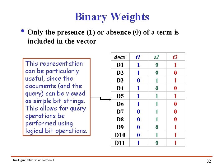
Binary Weights i Only the presence (1) or absence (0) of a term is included in the vector This representation can be particularly useful, since the documents (and the query) can be viewed as simple bit strings. This allows for query operations be performed using logical bit operations. Intelligent Information Retrieval 32

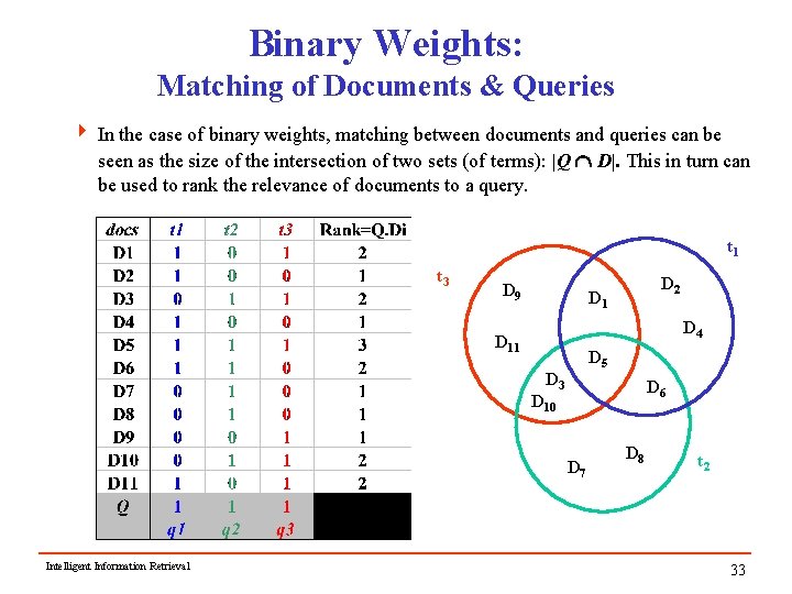
Binary Weights: Matching of Documents & Queries 4 In the case of binary weights, matching between documents and queries can be seen as the size of the intersection of two sets (of terms): |Q Ç D|. This in turn can be used to rank the relevance of documents to a query. t 1 t 3 D 9 D 2 D 1 D 4 D 11 D 5 D 3 D 6 D 10 D 7 Intelligent Information Retrieval D 8 t 2 33

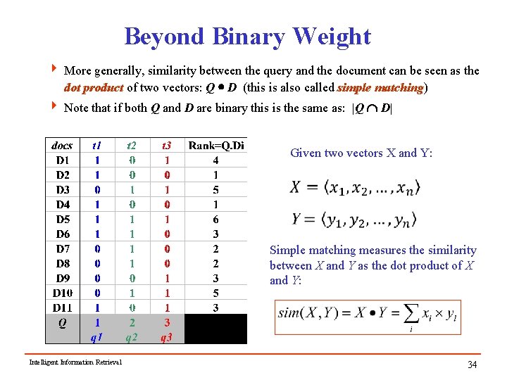
Beyond Binary Weight 4 More generally, similarity between the query and the document can be seen as the dot product of two vectors: Q · D (this is also called simple matching) 4 Note that if both Q and D are binary this is the same as: |Q Ç D| Given two vectors X and Y: Simple matching measures the similarity between X and Y as the dot product of X and Y: Intelligent Information Retrieval 34

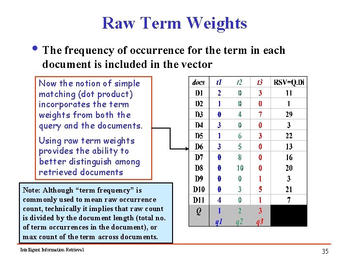
Raw Term Weights i The frequency of occurrence for the term in each document is included in the vector Now the notion of simple matching (dot product) incorporates the term weights from both the query and the documents. Using raw term weights provides the ability to better distinguish among retrieved documents Note: Although “term frequency” is commonly used to mean raw occurrence count, technically it implies that raw count is divided by the document length (total no. of term occurrences in the document), or max count of the term across documents. Intelligent Information Retrieval 35

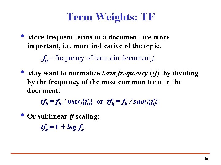
Term Weights: TF i More frequent terms in a document are more important, i. e. more indicative of the topic. fij = frequency of term i in document j. i May want to normalize term frequency (tf) by dividing by the frequency of the most common term in the document: tfij = fij / maxi{fij} or tfij = fij / sumi{fij} i Or sublinear tf scaling: tfij = 1 + log fij 36

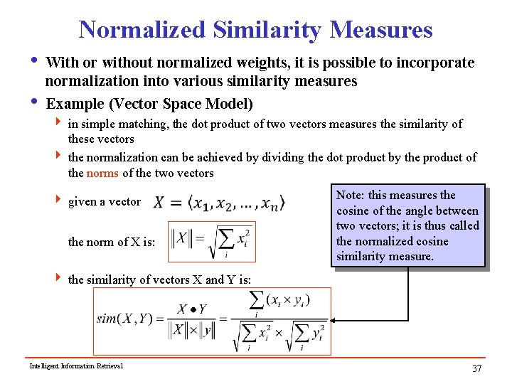
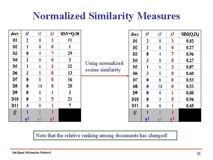
Normalized Similarity Measures i With or without normalized weights, it is possible to incorporate normalization into various similarity measures i Example (Vector Space Model) 4 in simple matching, the dot product of two vectors measures the similarity of these vectors 4 the normalization can be achieved by dividing the dot product by the product of the norms of the two vectors 4 given a vector the norm of X is: Note: this measures the cosine of the angle between two vectors; it is thus called the normalized cosine similarity measure. 4 the similarity of vectors X and Y is: Intelligent Information Retrieval 37

Normalized Similarity Measures Using normalized cosine similarity Note that the relative ranking among documents has changed! Intelligent Information Retrieval 38

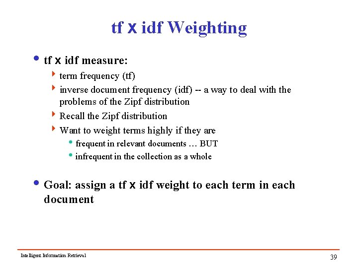
tf x idf Weighting i tf x idf measure: 4 term frequency (tf) 4 inverse document frequency (idf) -- a way to deal with the problems of the Zipf distribution 4 Recall the Zipf distribution 4 Want to weight terms highly if they are ifrequent in relevant documents … BUT iinfrequent in the collection as a whole i Goal: assign a tf x idf weight to each term in each document Intelligent Information Retrieval 39

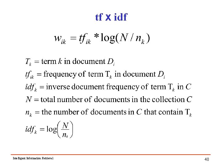
tf x idf Intelligent Information Retrieval 40

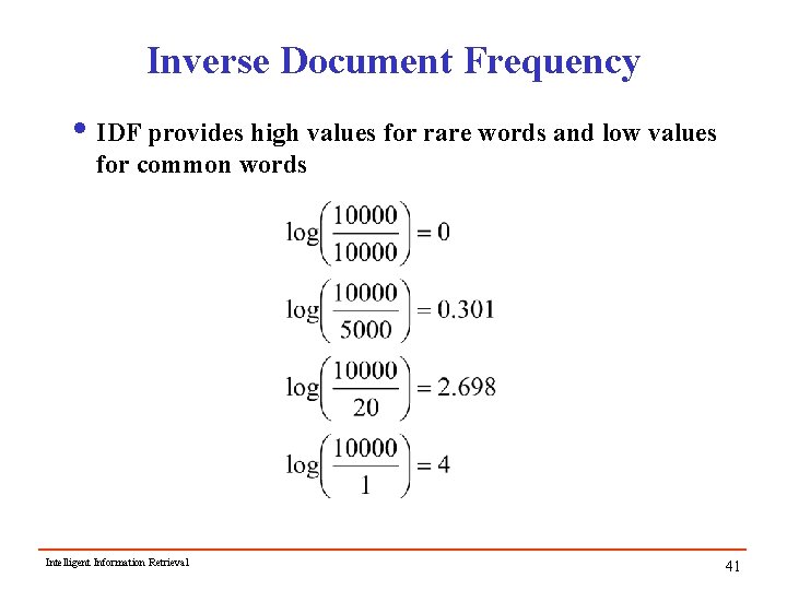
Inverse Document Frequency i IDF provides high values for rare words and low values for common words Intelligent Information Retrieval 41

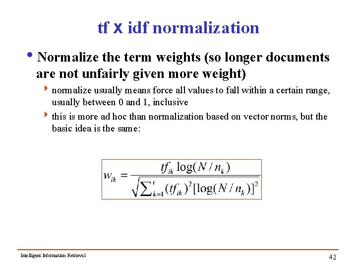
tf x idf normalization i. Normalize the term weights (so longer documents are not unfairly given more weight) 4 normalize usually means force all values to fall within a certain range, usually between 0 and 1, inclusive 4 this is more ad hoc than normalization based on vector norms, but the basic idea is the same: Intelligent Information Retrieval 42

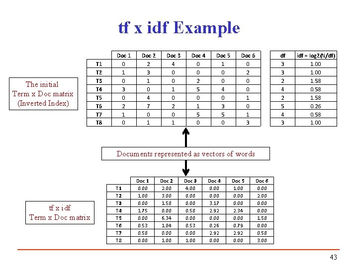
tf x idf Example The initial Term x Doc matrix (Inverted Index) T 1 T 2 T 3 T 4 T 5 T 6 T 7 T 8 Doc 1 0 3 0 2 1 0 Doc 2 2 3 1 0 4 7 0 1 Doc 3 4 0 0 1 0 2 0 1 Doc 4 0 0 2 5 0 1 5 0 Doc 5 1 0 0 4 0 3 5 0 Doc 6 0 2 0 0 1 3 df 3 3 2 4 2 5 4 3 idf = log 2(N/df) 1. 00 1. 58 0. 58 1. 58 0. 26 0. 58 1. 00 Documents represented as vectors of words tf x idf Term x Doc matrix T 1 T 2 T 3 T 4 T 5 T 6 T 7 T 8 Doc 1 0. 00 1. 00 0. 00 1. 75 0. 00 0. 53 0. 58 0. 00 Doc 2 2. 00 3. 00 1. 58 0. 00 6. 34 1. 84 0. 00 1. 00 Doc 3 4. 00 0. 58 0. 00 0. 53 0. 00 1. 00 Doc 4 0. 00 3. 17 2. 92 0. 00 0. 26 2. 92 0. 00 Doc 5 1. 00 0. 00 2. 34 0. 00 0. 79 2. 92 0. 00 Doc 6 0. 00 2. 00 0. 00 1. 58 0. 00 0. 58 3. 00 43

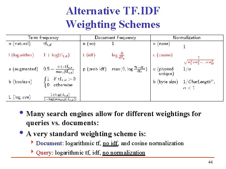
Alternative TF. IDF Weighting Schemes i Many search engines allow for different weightings for queries vs. documents: i A very standard weighting scheme is: 4 Document: logarithmic tf, no idf, and cosine normalization 4 Query: logarithmic tf, idf, no normalization 44

Keyword Discrimination Model i The Vector representation of documents can be used as the source of another approach to term weighting 4 Question: what happens if we removed one of the words used as dimensions in the vector space? 4 If the average similarity among documents changes significantly, then the word was a good discriminator 4 If there is little change, the word is not as helpful and should be weighted less i Note that the goal is to have a representation that makes it easier for a queries to discriminate among documents i Average similarity can be measured after removing each word from the matrix 4 Any of the similarity measures can be used (we will look at a variety of other similarity measures later). Intelligent Information Retrieval 45

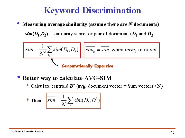
Keyword Discrimination i Measuring average similarity (assume there are N documents) sim(D 1, D 2) = similarity score for pair of documents D 1 and D 2 Computationally Expensive i Better way to calculate AVG-SIM 4 Calculate centroid D* (avg. document vector = Sum vectors / N) 4 Then: Intelligent Information Retrieval 46

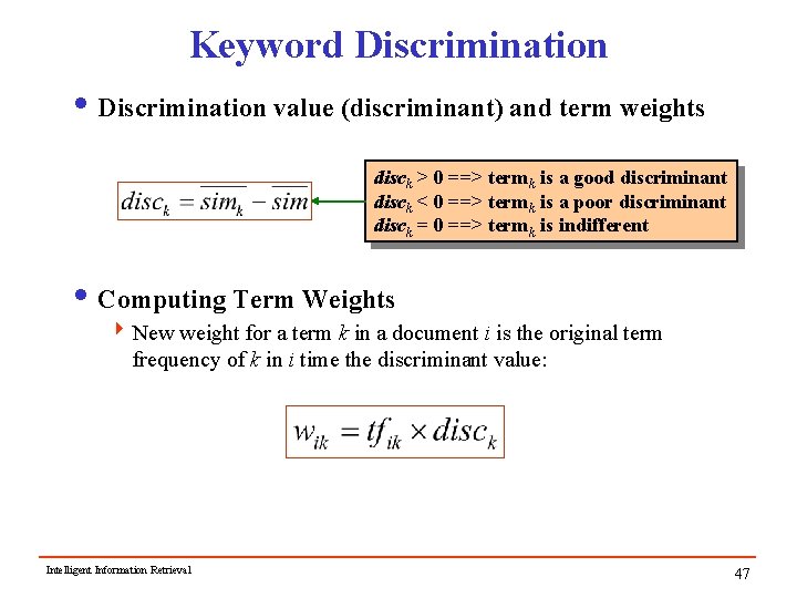
Keyword Discrimination i Discrimination value (discriminant) and term weights disck > 0 ==> termk is a good discriminant disck < 0 ==> termk is a poor discriminant disck = 0 ==> termk is indifferent i Computing Term Weights 4 New weight for a term k in a document i is the original term frequency of k in i time the discriminant value: Intelligent Information Retrieval 47

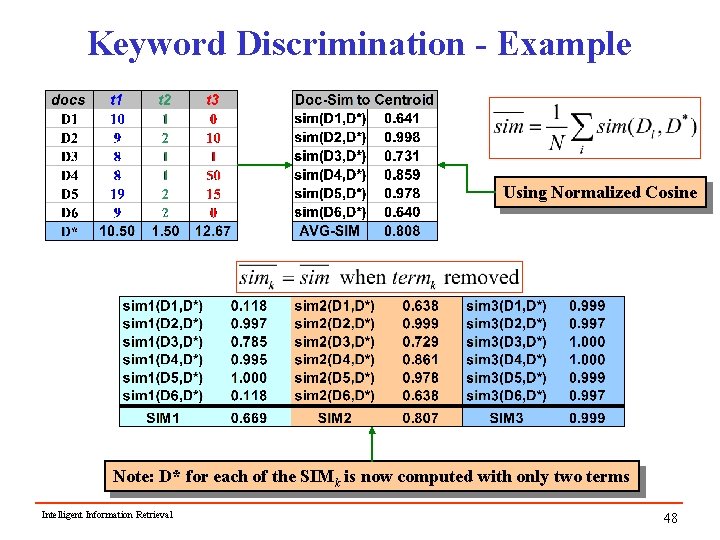
Keyword Discrimination - Example Using Normalized Cosine Note: D* for each of the SIMk is now computed with only two terms Intelligent Information Retrieval 48

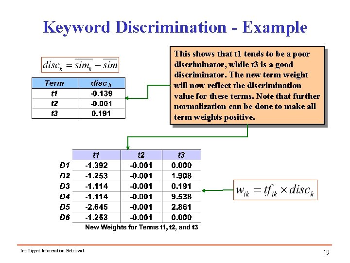
Keyword Discrimination - Example This shows that t 1 tends to be a poor discriminator, while t 3 is a good discriminator. The new term weight will now reflect the discrimination value for these terms. Note that further normalization can be done to make all term weights positive. Intelligent Information Retrieval 49

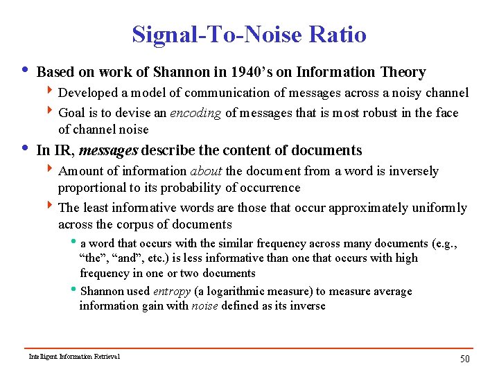
Signal-To-Noise Ratio i Based on work of Shannon in 1940’s on Information Theory 4 Developed a model of communication of messages across a noisy channel 4 Goal is to devise an encoding of messages that is most robust in the face of channel noise i In IR, messages describe the content of documents 4 Amount of information about the document from a word is inversely proportional to its probability of occurrence 4 The least informative words are those that occur approximately uniformly across the corpus of documents ia word that occurs with the similar frequency across many documents (e. g. , “the”, “and”, etc. ) is less informative than one that occurs with high frequency in one or two documents i. Shannon used entropy (a logarithmic measure) to measure average information gain with noise defined as its inverse Intelligent Information Retrieval 50

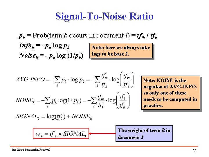
Signal-To-Noise Ratio pk = Prob(term k occurs in document i) = tfik / tfk Infok = - pk log pk Note: here we always take Noisek = - pk log (1/pk) logs to be base 2. Note: NOISE is the negation of AVG-INFO, so only one of these needs to be computed in practice. The weight of term k in document i Intelligent Information Retrieval 51

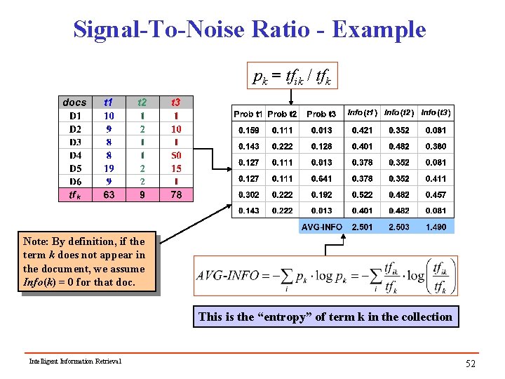
Signal-To-Noise Ratio - Example pk = tfik / tfk Note: By definition, if the term k does not appear in the document, we assume Info(k) = 0 for that doc. This is the “entropy” of term k in the collection Intelligent Information Retrieval 52

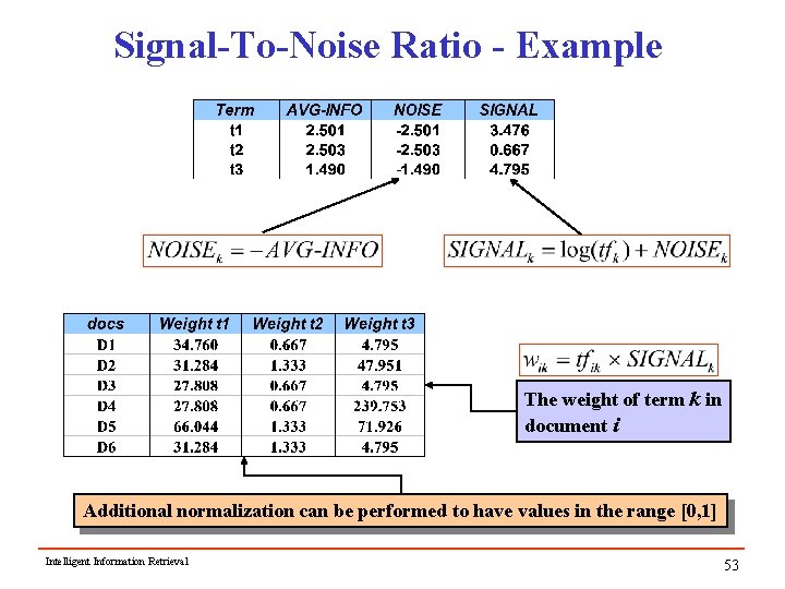
Signal-To-Noise Ratio - Example The weight of term k in document i Additional normalization can be performed to have values in the range [0, 1] Intelligent Information Retrieval 53

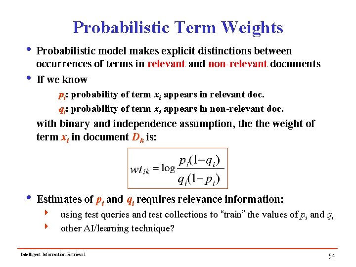
Probabilistic Term Weights i Probabilistic model makes explicit distinctions between occurrences of terms in relevant and non-relevant documents i If we know pi: probability of term xi appears in relevant doc. qi: probability of term xi appears in non-relevant doc. with binary and independence assumption, the weight of term xi in document Dk is: i Estimates of pi and qi requires relevance information: 4 using test queries and test collections to “train” the values of pi and qi 4 other AI/learning technique? Intelligent Information Retrieval 54

Phrase Indexing and Phrase Queries i Both statistical and syntactic methods have been used to identify “good” phrases 4 Example: Mutual Expected Information to find “co-locations” 4 Linguistic Approaches: using a part-of-speech tagger to identify simple noun phrases i Phrases can have an impact on effectiveness and efficiency 4 phrase indexing will speed up phrase queries 4 improve precision by disambiguating the word senses: ie. g, “grass field” v. “magnetic field” 4 effectiveness not straightforward and depends on retrieval model ie. g. “information retrieval”, how much do individual words count? • For phrase queries, it no longer suffices to store only <term : docs> entries Intelligent Information Retrieval 55

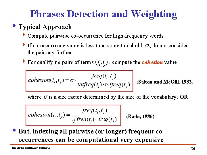
Phrases Detection and Weighting i Typical Approach 4 Compute pairwise co-occurrence for high-frequency words 4 If co-occurrence value is less than some threshold a, do not consider the pair any further 4 For qualifying pairs of terms (ti, tj) , compute the cohesion value (Salton and Mc. Gill, 1983) where s is a size factor determined by the size of the vocabulary; OR (Rada, 1986) i But, indexing all pairwise (or longer) frequent cooccurrences can be computational very expensive Intelligent Information Retrieval 56

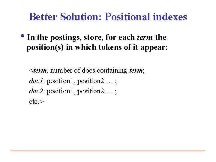
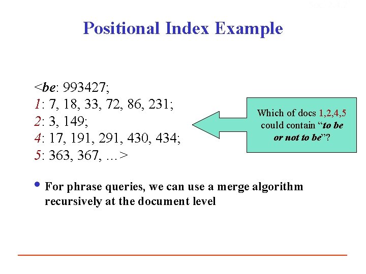
Sec. 2. 4. 2 Better Solution: Positional indexes i. In the postings, store, for each term the position(s) in which tokens of it appear: <term, number of docs containing term; doc 1: position 1, position 2 … ; doc 2: position 1, position 2 … ; etc. >

Sec. 2. 4. 2 Positional Index Example <be: 993427; 1: 7, 18, 33, 72, 86, 231; 2: 3, 149; 4: 17, 191, 291, 430, 434; 5: 363, 367, …> Which of docs 1, 2, 4, 5 could contain “to be or not to be”? i For phrase queries, we can use a merge algorithm recursively at the document level

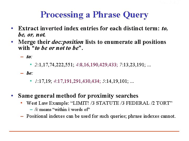
Sec. 2. 4. 2 Processing a Phrase Query • Extract inverted index entries for each distinct term: to, be, or, not. • Merge their doc: position lists to enumerate all positions with “to be or not to be”. – to: • 2: 1, 17, 74, 222, 551; 4: 8, 16, 190, 429, 433; 7: 13, 23, 191; . . . – be: • 1: 17, 19; 4: 17, 191, 291, 430, 434; 5: 14, 19, 101; . . . • Same general method for proximity searches • West Law Example: “LIMIT! /3 STATUTE /3 FEDERAL /2 TORT” – /k means “within k words of” – Positional indexes can be used for such queries; phrase indexes cannot.

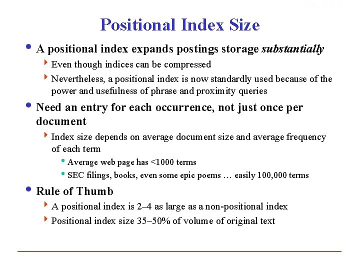
Sec. 2. 4. 2 Positional Index Size i A positional index expands postings storage substantially 4 Even though indices can be compressed 4 Nevertheless, a positional index is now standardly used because of the power and usefulness of phrase and proximity queries i Need an entry for each occurrence, not just once per document 4 Index size depends on average document size and average frequency of each term i. Average web page has <1000 terms i. SEC filings, books, even some epic poems … easily 100, 000 terms i Rule of Thumb 4 A positional index is 2– 4 as large as a non-positional index 4 Positional index size 35– 50% of volume of original text

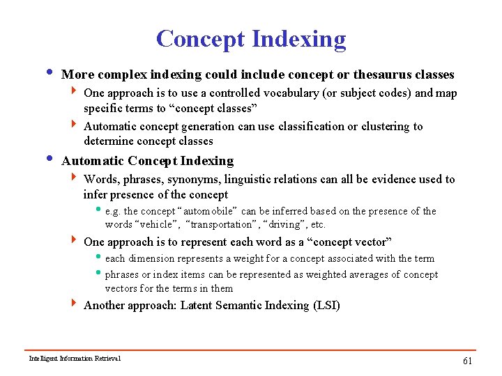
Concept Indexing i More complex indexing could include concept or thesaurus classes 4 One approach is to use a controlled vocabulary (or subject codes) and map specific terms to “concept classes” 4 Automatic concept generation can use classification or clustering to determine concept classes i Automatic Concept Indexing 4 Words, phrases, synonyms, linguistic relations can all be evidence used to infer presence of the concept i e. g. the concept “automobile” can be inferred based on the presence of the words “vehicle”, “transportation”, “driving”, etc. 4 One approach is to represent each word as a “concept vector” i each dimension represents a weight for a concept associated with the term i phrases or index items can be represented as weighted averages of concept vectors for the terms in them 4 Another approach: Latent Semantic Indexing (LSI) Intelligent Information Retrieval 61

Next i Retrieval Models and Ranking Algorithms 4 Boolean Matching and Boolean Queries 4 Vector Space Model and Similarity Ranking 4 Extended Boolean Models 4 Basic Probabilistic Models 4 Implementation Issues for Ranking Systems Intelligent Information Retrieval 62