CS 267 Applications of Parallel Computers Lecture 17

CS 267: Applications of Parallel Computers Lecture 17 - Structured Grids James Demmel www. cs. berkeley. edu/~demmel/cs 267_Spr 15

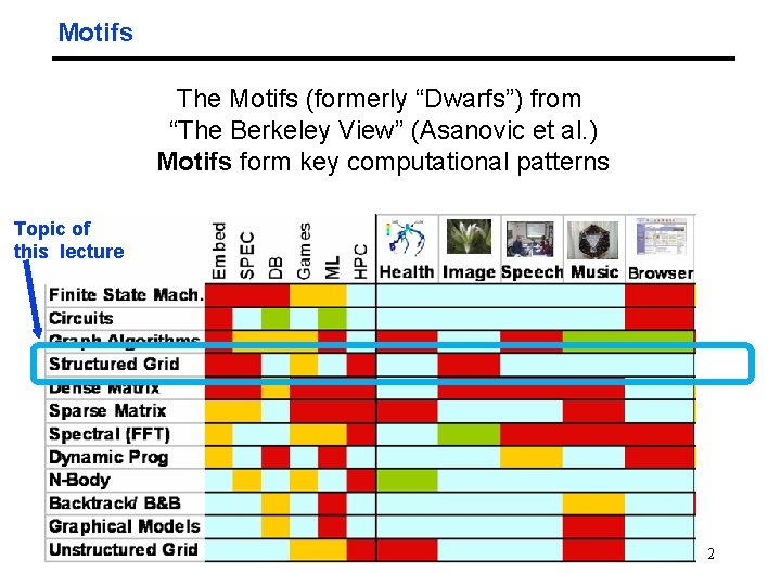
Motifs The Motifs (formerly “Dwarfs”) from “The Berkeley View” (Asanovic et al. ) Motifs form key computational patterns Topic of this lecture 03/13/12 CS 267 Lecture 2 17 2

Outline ° Review of Poisson Equation ° Jacobi’s method ° Red-Black SOR method ° Conjugate Gradient (topic of Lecture 16) ° Multigrid ° (Later lecture: FFTs) 03/17/2015 CS 267 Lecture 17 3

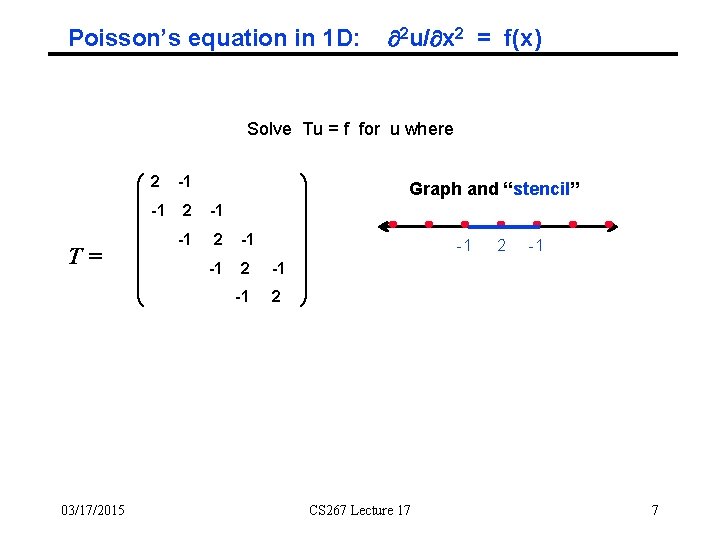
Poisson’s equation in 1 D: 2 u/ x 2 = f(x) Solve Tu = f for u where T= 03/17/2015 2 -1 -1 2 Graph and “stencil” -1 CS 267 Lecture 17 2 -1 7

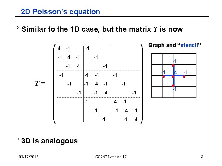
2 D Poisson’s equation ° Similar to the 1 D case, but the matrix T is now 4 -1 -1 4 -1 T= Graph and “stencil” -1 -1 -1 4 -1 -1 -1 4 -1 -1 4 ° 3 D is analogous 03/17/2015 CS 267 Lecture 17 8

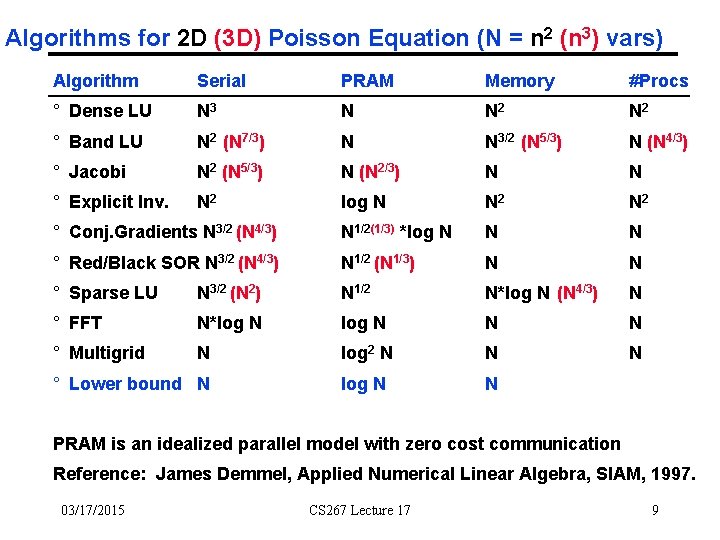
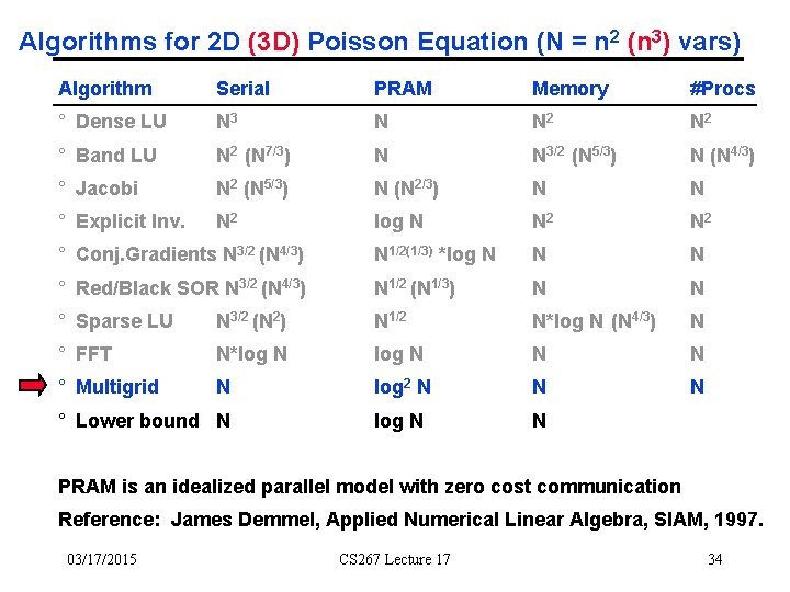
Algorithms for 2 D (3 D) Poisson Equation (N = n 2 (n 3) vars) Algorithm Serial PRAM Memory #Procs ° Dense LU N 3 N N 2 ° Band LU N 2 (N 7/3) N N 3/2 (N 5/3) N (N 4/3) ° Jacobi N 2 (N 5/3) N (N 2/3) N N ° Explicit Inv. N 2 log N N 2 ° Conj. Gradients N 3/2 (N 4/3) N 1/2(1/3) *log N N N ° Red/Black SOR N 3/2 (N 4/3) N 1/2 (N 1/3) N N ° Sparse LU N 3/2 (N 2) N 1/2 N*log N (N 4/3) N ° FFT N*log N N N ° Multigrid N log 2 N N N log N N ° Lower bound N PRAM is an idealized parallel model with zero cost communication Reference: James Demmel, Applied Numerical Linear Algebra, SIAM, 1997. 03/17/2015 CS 267 Lecture 17 9

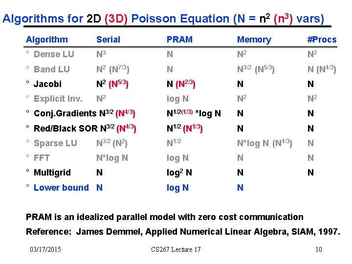
Algorithms for 2 D (3 D) Poisson Equation (N = n 2 (n 3) vars) Algorithm Serial PRAM Memory #Procs ° Dense LU N 3 N N 2 ° Band LU N 2 (N 7/3) N N 3/2 (N 5/3) N (N 4/3) ° Jacobi N 2 (N 5/3) N (N 2/3) N N ° Explicit Inv. N 2 log N N 2 ° Conj. Gradients N 3/2 (N 4/3) N 1/2(1/3) *log N N N ° Red/Black SOR N 3/2 (N 4/3) N 1/2 (N 1/3) N N ° Sparse LU N 3/2 (N 2) N 1/2 N*log N (N 4/3) N ° FFT N*log N N N ° Multigrid N log 2 N N N log N N ° Lower bound N PRAM is an idealized parallel model with zero cost communication Reference: James Demmel, Applied Numerical Linear Algebra, SIAM, 1997. 03/17/2015 CS 267 Lecture 17 10

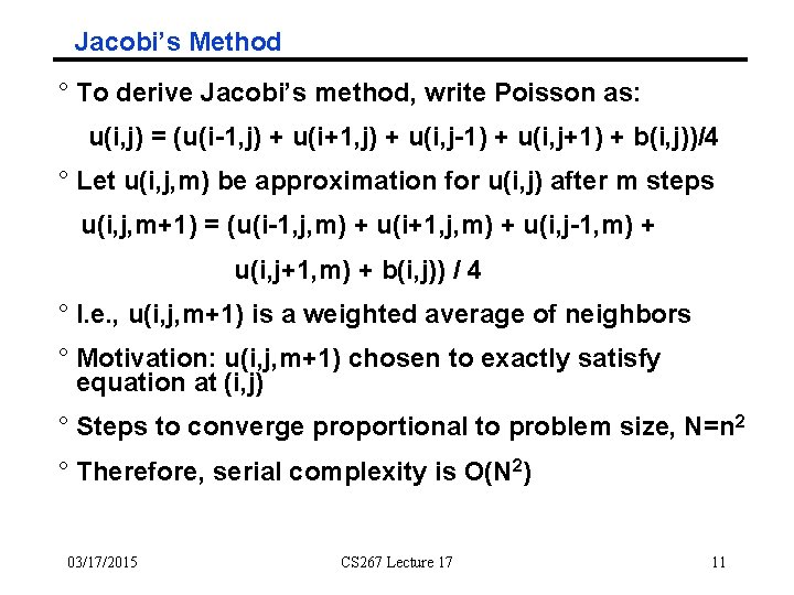
Jacobi’s Method ° To derive Jacobi’s method, write Poisson as: u(i, j) = (u(i-1, j) + u(i+1, j) + u(i, j-1) + u(i, j+1) + b(i, j))/4 ° Let u(i, j, m) be approximation for u(i, j) after m steps u(i, j, m+1) = (u(i-1, j, m) + u(i+1, j, m) + u(i, j-1, m) + u(i, j+1, m) + b(i, j)) / 4 ° I. e. , u(i, j, m+1) is a weighted average of neighbors ° Motivation: u(i, j, m+1) chosen to exactly satisfy equation at (i, j) ° Steps to converge proportional to problem size, N=n 2 ° Therefore, serial complexity is O(N 2) 03/17/2015 CS 267 Lecture 17 11

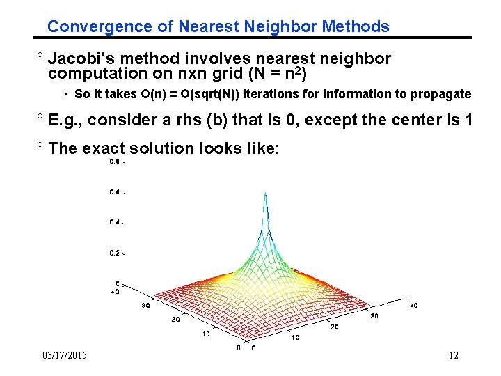
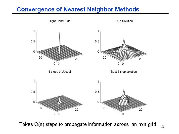
Convergence of Nearest Neighbor Methods ° Jacobi’s method involves nearest neighbor computation on nxn grid (N = n 2) • So it takes O(n) = O(sqrt(N)) iterations for information to propagate ° E. g. , consider a rhs (b) that is 0, except the center is 1 ° The exact solution looks like: 03/17/2015 12

Convergence of Nearest Neighbor Methods Takes O(n) steps to propagate information across an nxn grid 13

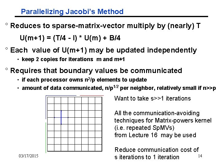
Parallelizing Jacobi’s Method ° Reduces to sparse-matrix-vector multiply by (nearly) T U(m+1) = (T/4 - I) * U(m) + B/4 ° Each value of U(m+1) may be updated independently • keep 2 copies for iterations m and m+1 ° Requires that boundary values be communicated • if each processor owns n 2/p elements to update • amount of data communicated, n/p 1/2 per neighbor, relatively small if n>>p Want to take s>>1 iterations All the communication-avoiding techniques for Matrix-powers kernel (i. e. repeated Sp. MVs) from Lecture 16 may be used 03/17/2015 Reduce communication cost of 14 s iterations to 1 iteration

References for Optimizing Stencils (1/2) ° Bebop. cs. berkeley. edu • “Autotuning Stencil Codes for Cache-Based Multicore Platforms”, Datta, UCB Ph. D thesis, 2009, • “Avoiding Communication in Computing Krylov Subspaces, ” Demmel, M. Hoemmen, M. Mohiyuddin, K. Yelick, 2007 • “Optimization and Performance Modeling of Stencil Computations on Modern Microprocessors”, K. Datta, S. Kamil, S. Williams, L. Oliker, J. Shalf, K. Yelick, SIAM Review, 2008 ° SEJITS – sejits. org (Armando Fox et al @ UCB) “Bringing parallel performance to python with domainspecific selective embedded just-in-time specialization” ° Pochoir – stencil compiler (Charles Leiserson @ MIT) people. csail. mit. edu/yuantang/ ° Autotuning stencils and multigrid (Mary Hall @ Utah) super-scidac. org/ ° Polyhedral tiling (Michelle Strout @ Colorado) www. cs. colostate. edu/~mstrout/Papers/pubs-poly. php

References for Optimizing Stencils (2/2) ° Ian Foster et al, on grids (SC 2001) ° “Efficient out-of-core algorithms for linear relaxation using blocking covers, ” C. Leiserson, S. Rao, S. Toledo, FOCS, 1993 ° “Data flow and storage allocation for the PDQ-5 program on the Philco-2000, ” C. Pfeifer, CACM, 1963

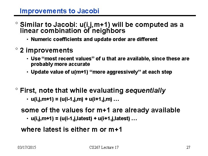
Improvements to Jacobi ° Similar to Jacobi: u(i, j, m+1) will be computed as a linear combination of neighbors • Numeric coefficients and update order are different ° 2 improvements • Use “most recent values” of u that are available, since these are probably more accurate • Update value of u(m+1) “more aggressively” at each step ° First, note that while evaluating sequentially • u(i, j, m+1) = (u(i-1, j, m) + u(i+1, j, m) … some of the values for m+1 are already available • u(i, j, m+1) = (u(i-1, j, latest) + u(i+1, j, latest) … where latest is either m or m+1 03/17/2015 CS 267 Lecture 17 27

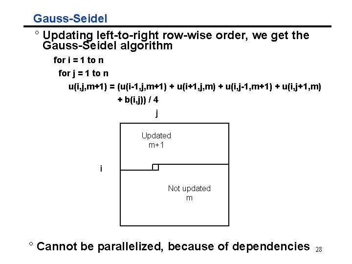
Gauss-Seidel ° Updating left-to-right row-wise order, we get the Gauss-Seidel algorithm for i = 1 to n for j = 1 to n u(i, j, m+1) = (u(i-1, j, m+1) + u(i+1, j, m) + u(i, j-1, m+1) + u(i, j+1, m) + b(i, j)) / 4 j Updated m+1 i Not updated m ° Cannot be parallelized, because of dependencies 28

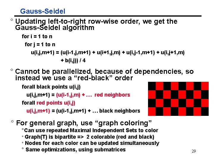
Gauss-Seidel ° Updating left-to-right row-wise order, we get the Gauss-Seidel algorithm for i = 1 to n for j = 1 to n u(i, j, m+1) = (u(i-1, j, m+1) + u(i+1, j, m) + u(i, j-1, m+1) + u(i, j+1, m) + b(i, j)) / 4 ° Cannot be parallelized, because of dependencies, so instead we use a “red-black” order forall black points u(i, j) u(i, j, m+1) = (u(i-1, j, m) + … red neighbors forall red points u(i, j) u(i, j, m+1) = (u(i-1, j, m+1) + … black neighbors ° For general graph, use “graph coloring” °Can use repeated Maximal Independent Sets to color ° Graph(T) is bipartite => 2 colorable (red and black) ° Nodes for each color can be updated simultaneously ° Same optimizations, using submatrices 29

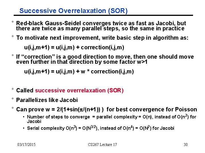
Successive Overrelaxation (SOR) ° Red-black Gauss-Seidel converges twice as fast as Jacobi, but there are twice as many parallel steps, so the same in practice ° To motivate next improvement, write basic step in algorithm as: u(i, j, m+1) = u(i, j, m) + correction(i, j, m) ° If “correction” is a good direction to move, then one should move even further in that direction by some factor w>1 u(i, j, m+1) = u(i, j, m) + w * correction(i, j, m) ° Called successive overrelaxation (SOR) ° Parallelizes like Jacobi ° Can prove w = 2/(1+sin(p/(n+1)) ) for best convergence for Poisson • Number of steps to converge = parallel complexity = O(n), instead of O(n 2) for Jacobi • Serial complexity O(n 3) = O(N 3/2), instead of O(n 4) = O(N 2) for Jacobi 03/17/2015 CS 267 Lecture 17 30

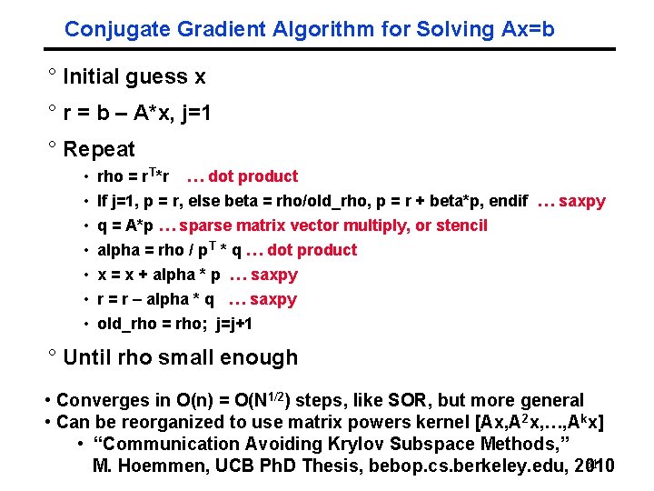
Conjugate Gradient Algorithm for Solving Ax=b ° Initial guess x ° r = b – A*x, j=1 ° Repeat • • rho = r. T*r … dot product If j=1, p = r, else beta = rho/old_rho, p = r + beta*p, endif … saxpy q = A*p … sparse matrix vector multiply, or stencil alpha = rho / p. T * q … dot product x = x + alpha * p … saxpy r = r – alpha * q … saxpy old_rho = rho; j=j+1 ° Until rho small enough • Converges in O(n) = O(N 1/2) steps, like SOR, but more general • Can be reorganized to use matrix powers kernel [Ax, A 2 x, …, Akx] • “Communication Avoiding Krylov Subspace Methods, ” 31 M. Hoemmen, UCB Ph. D Thesis, bebop. cs. berkeley. edu, 2010

Algorithms for 2 D (3 D) Poisson Equation (N = n 2 (n 3) vars) Algorithm Serial PRAM Memory #Procs ° Dense LU N 3 N N 2 ° Band LU N 2 (N 7/3) N N 3/2 (N 5/3) N (N 4/3) ° Jacobi N 2 (N 5/3) N (N 2/3) N N ° Explicit Inv. N 2 log N N 2 ° Conj. Gradients N 3/2 (N 4/3) N 1/2(1/3) *log N N N ° Red/Black SOR N 3/2 (N 4/3) N 1/2 (N 1/3) N N ° Sparse LU N 3/2 (N 2) N 1/2 N*log N (N 4/3) N ° FFT N*log N N N ° Multigrid N log 2 N N N log N N ° Lower bound N PRAM is an idealized parallel model with zero cost communication Reference: James Demmel, Applied Numerical Linear Algebra, SIAM, 1997. 03/17/2015 CS 267 Lecture 17 34

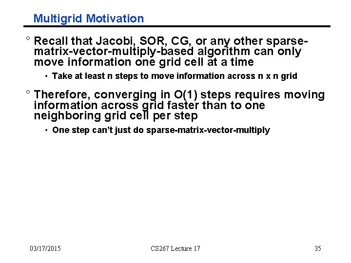
Multigrid Motivation ° Recall that Jacobi, SOR, CG, or any other sparsematrix-vector-multiply-based algorithm can only move information one grid cell at a time • Take at least n steps to move information across n x n grid ° Therefore, converging in O(1) steps requires moving information across grid faster than to one neighboring grid cell per step • One step can’t just do sparse-matrix-vector-multiply 03/17/2015 CS 267 Lecture 17 35

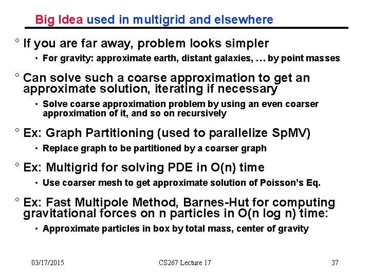
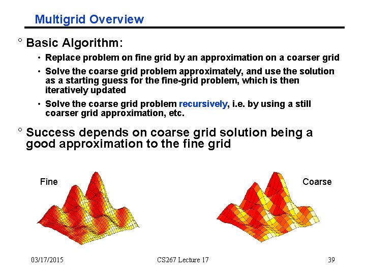
Big Idea used in multigrid and elsewhere ° If you are far away, problem looks simpler • For gravity: approximate earth, distant galaxies, … by point masses ° Can solve such a coarse approximation to get an approximate solution, iterating if necessary • Solve coarse approximation problem by using an even coarser approximation of it, and so on recursively ° Ex: Graph Partitioning (used to parallelize Sp. MV) • Replace graph to be partitioned by a coarser graph ° Ex: Multigrid for solving PDE in O(n) time • Use coarser mesh to get approximate solution of Poisson’s Eq. ° Ex: Fast Multipole Method, Barnes-Hut for computing gravitational forces on n particles in O(n log n) time: • Approximate particles in box by total mass, center of gravity 03/17/2015 CS 267 Lecture 17 37

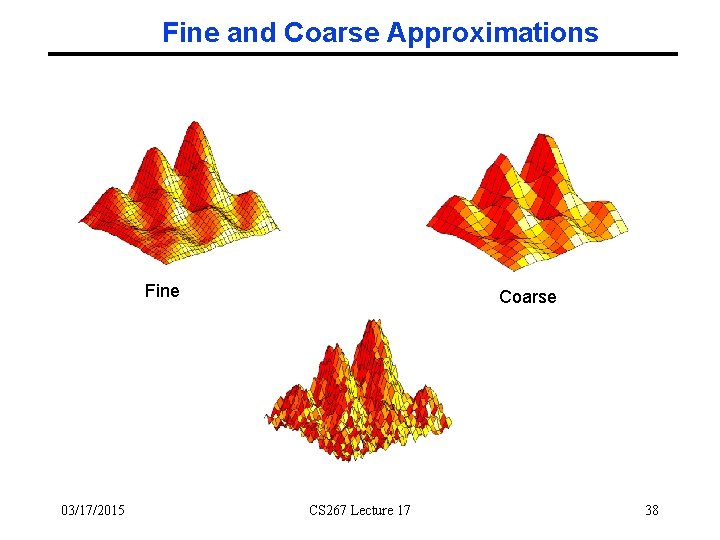
Fine and Coarse Approximations Fine 03/17/2015 Coarse CS 267 Lecture 17 38

Multigrid Overview ° Basic Algorithm: • Replace problem on fine grid by an approximation on a coarser grid • Solve the coarse grid problem approximately, and use the solution as a starting guess for the fine-grid problem, which is then iteratively updated • Solve the coarse grid problem recursively, i. e. by using a still coarser grid approximation, etc. ° Success depends on coarse grid solution being a good approximation to the fine grid Fine 03/17/2015 Coarse CS 267 Lecture 17 39

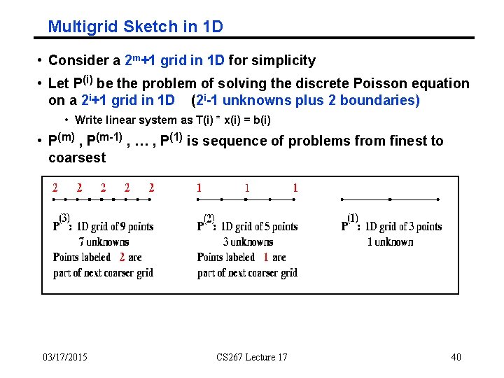
Multigrid Sketch in 1 D • Consider a 2 m+1 grid in 1 D for simplicity • Let P(i) be the problem of solving the discrete Poisson equation on a 2 i+1 grid in 1 D (2 i-1 unknowns plus 2 boundaries) • • Write linear system as T(i) * x(i) = b(i) P(m) , P(m-1) , … , P(1) is sequence of problems from finest to coarsest 03/17/2015 CS 267 Lecture 17 40

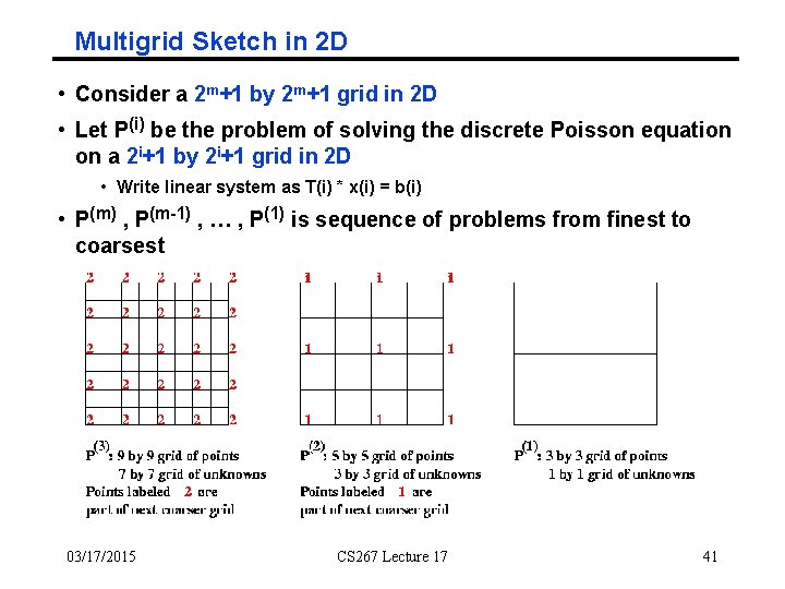
Multigrid Sketch in 2 D • Consider a 2 m+1 by 2 m+1 grid in 2 D • Let P(i) be the problem of solving the discrete Poisson equation on a 2 i+1 by 2 i+1 grid in 2 D • • Write linear system as T(i) * x(i) = b(i) P(m) , P(m-1) , … , P(1) is sequence of problems from finest to coarsest 03/17/2015 CS 267 Lecture 17 41

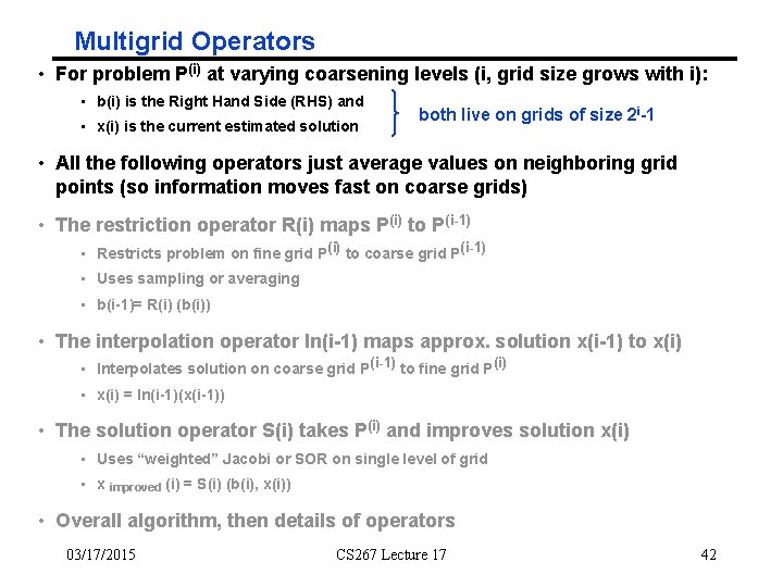
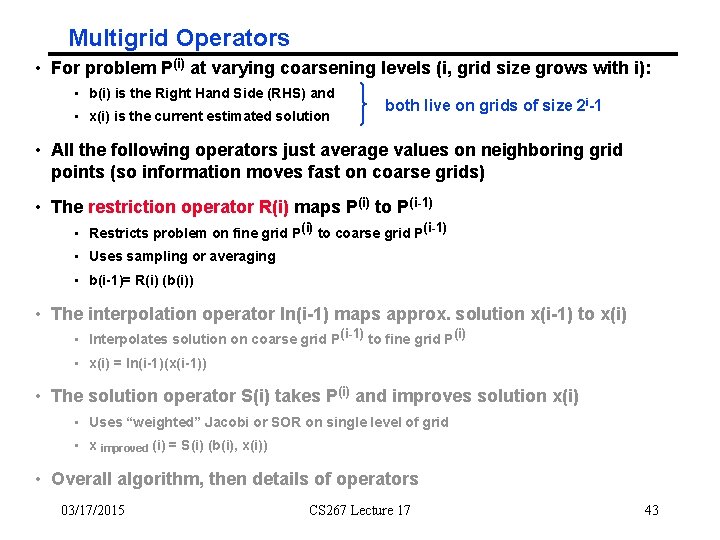
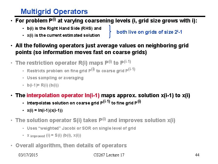
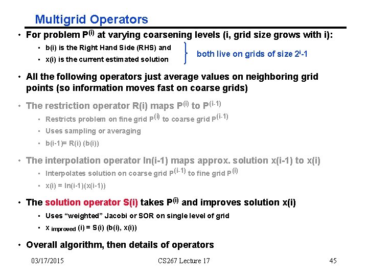
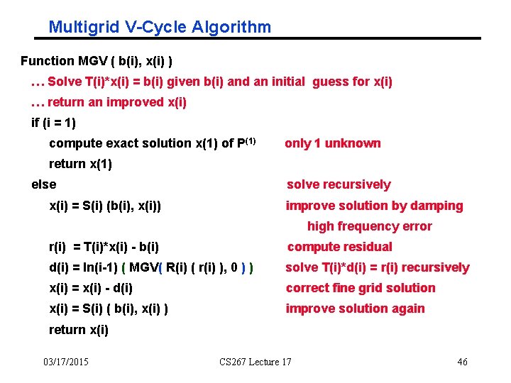
Multigrid Operators • For problem P(i) at varying coarsening levels (i, grid size grows with i): • b(i) is the Right Hand Side (RHS) and • x(i) is the current estimated solution both live on grids of size 2 i-1 • All the following operators just average values on neighboring grid points (so information moves fast on coarse grids) • The restriction operator R(i) maps P(i) to P(i-1) • Restricts problem on fine grid P(i) to coarse grid P(i-1) • Uses sampling or averaging • b(i-1)= R(i) (b(i)) • The interpolation operator In(i-1) maps approx. solution x(i-1) to x(i) • Interpolates solution on coarse grid P(i-1) to fine grid P(i) • x(i) = In(i-1)(x(i-1)) • The solution operator S(i) takes P(i) and improves solution x(i) • Uses “weighted” Jacobi or SOR on single level of grid • x improved (i) = S(i) (b(i), x(i)) • Overall algorithm, then details of operators 03/17/2015 CS 267 Lecture 17 42

Multigrid Operators • For problem P(i) at varying coarsening levels (i, grid size grows with i): • b(i) is the Right Hand Side (RHS) and • x(i) is the current estimated solution both live on grids of size 2 i-1 • All the following operators just average values on neighboring grid points (so information moves fast on coarse grids) • The restriction operator R(i) maps P(i) to P(i-1) • Restricts problem on fine grid P(i) to coarse grid P(i-1) • Uses sampling or averaging • b(i-1)= R(i) (b(i)) • The interpolation operator In(i-1) maps approx. solution x(i-1) to x(i) • Interpolates solution on coarse grid P(i-1) to fine grid P(i) • x(i) = In(i-1)(x(i-1)) • The solution operator S(i) takes P(i) and improves solution x(i) • Uses “weighted” Jacobi or SOR on single level of grid • x improved (i) = S(i) (b(i), x(i)) • Overall algorithm, then details of operators 03/17/2015 CS 267 Lecture 17 43

Multigrid Operators • For problem P(i) at varying coarsening levels (i, grid size grows with i): • b(i) is the Right Hand Side (RHS) and • x(i) is the current estimated solution both live on grids of size 2 i-1 • All the following operators just average values on neighboring grid points (so information moves fast on coarse grids) • The restriction operator R(i) maps P(i) to P(i-1) • Restricts problem on fine grid P(i) to coarse grid P(i-1) • Uses sampling or averaging • b(i-1)= R(i) (b(i)) • The interpolation operator In(i-1) maps approx. solution x(i-1) to x(i) • Interpolates solution on coarse grid P(i-1) to fine grid P(i) • x(i) = In(i-1)(x(i-1)) • The solution operator S(i) takes P(i) and improves solution x(i) • Uses “weighted” Jacobi or SOR on single level of grid • x improved (i) = S(i) (b(i), x(i)) • Overall algorithm, then details of operators 03/17/2015 CS 267 Lecture 17 44

Multigrid Operators • For problem P(i) at varying coarsening levels (i, grid size grows with i): • b(i) is the Right Hand Side (RHS) and • x(i) is the current estimated solution both live on grids of size 2 i-1 • All the following operators just average values on neighboring grid points (so information moves fast on coarse grids) • The restriction operator R(i) maps P(i) to P(i-1) • Restricts problem on fine grid P(i) to coarse grid P(i-1) • Uses sampling or averaging • b(i-1)= R(i) (b(i)) • The interpolation operator In(i-1) maps approx. solution x(i-1) to x(i) • Interpolates solution on coarse grid P(i-1) to fine grid P(i) • x(i) = In(i-1)(x(i-1)) • The solution operator S(i) takes P(i) and improves solution x(i) • Uses “weighted” Jacobi or SOR on single level of grid • x improved (i) = S(i) (b(i), x(i)) • Overall algorithm, then details of operators 03/17/2015 CS 267 Lecture 17 45

Multigrid V-Cycle Algorithm Function MGV ( b(i), x(i) ) … Solve T(i)*x(i) = b(i) given b(i) and an initial guess for x(i) … return an improved x(i) if (i = 1) compute exact solution x(1) of P(1) only 1 unknown return x(1) else solve recursively x(i) = S(i) (b(i), x(i)) improve solution by damping high frequency error r(i) = T(i)*x(i) - b(i) compute residual d(i) = In(i-1) ( MGV( R(i) ( r(i) ), 0 ) ) solve T(i)*d(i) = r(i) recursively x(i) = x(i) - d(i) correct fine grid solution x(i) = S(i) ( b(i), x(i) ) improve solution again return x(i) 03/17/2015 CS 267 Lecture 17 46

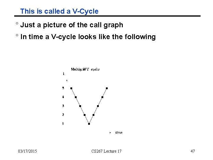
This is called a V-Cycle ° Just a picture of the call graph ° In time a V-cycle looks like the following 03/17/2015 CS 267 Lecture 17 47

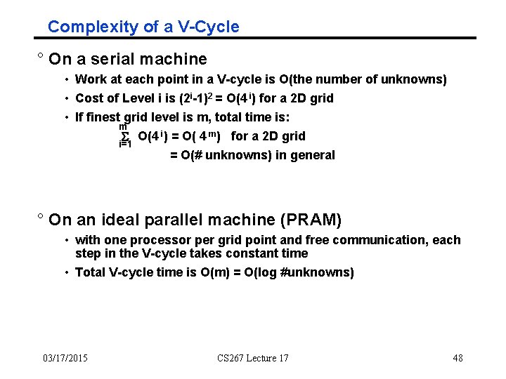
Complexity of a V-Cycle ° On a serial machine • Work at each point in a V-cycle is O(the number of unknowns) • Cost of Level i is (2 i-1)2 = O(4 i) for a 2 D grid • If finest grid level is m, total time is: m S O(4 i) = O( 4 m) for a 2 D grid i=1 = O(# unknowns) in general ° On an ideal parallel machine (PRAM) • with one processor per grid point and free communication, each step in the V-cycle takes constant time • Total V-cycle time is O(m) = O(log #unknowns) 03/17/2015 CS 267 Lecture 17 48

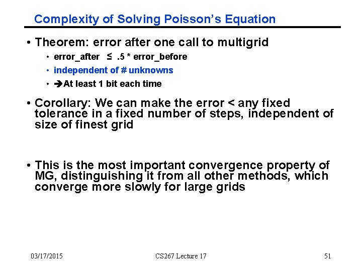
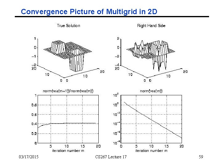
Complexity of Solving Poisson’s Equation • Theorem: error after one call to multigrid • error_after ≤. 5 * error_before • independent of # unknowns • At least 1 bit each time • Corollary: We can make the error < any fixed tolerance in a fixed number of steps, independent of size of finest grid • This is the most important convergence property of MG, distinguishing it from all other methods, which converge more slowly for large grids 03/17/2015 CS 267 Lecture 17 51

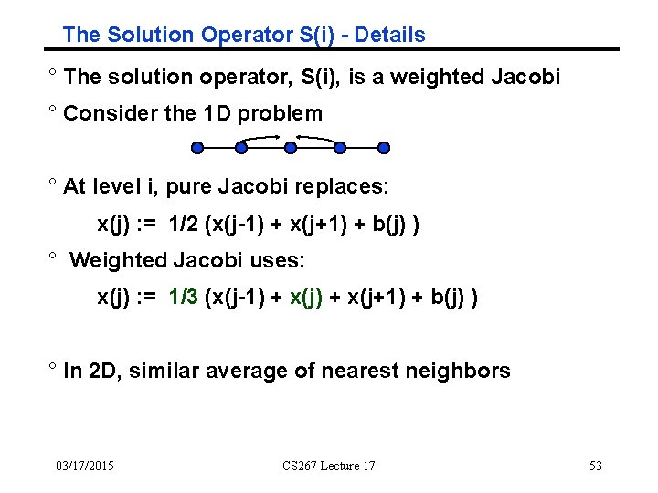
The Solution Operator S(i) - Details ° The solution operator, S(i), is a weighted Jacobi ° Consider the 1 D problem ° At level i, pure Jacobi replaces: x(j) : = 1/2 (x(j-1) + x(j+1) + b(j) ) ° Weighted Jacobi uses: x(j) : = 1/3 (x(j-1) + x(j+1) + b(j) ) ° In 2 D, similar average of nearest neighbors 03/17/2015 CS 267 Lecture 17 53

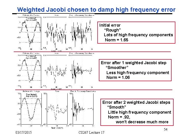
Weighted Jacobi chosen to damp high frequency error Initial error “Rough” Lots of high frequency components Norm = 1. 65 Error after 1 weighted Jacobi step “Smoother” Less high frequency component Norm = 1. 06 Error after 2 weighted Jacobi steps “Smooth” Little high frequency component Norm =. 92, won’t decrease much more 03/17/2015 CS 267 Lecture 17 54

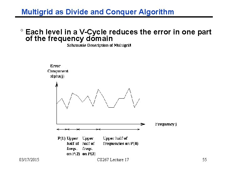
Multigrid as Divide and Conquer Algorithm ° Each level in a V-Cycle reduces the error in one part of the frequency domain 03/17/2015 CS 267 Lecture 17 55

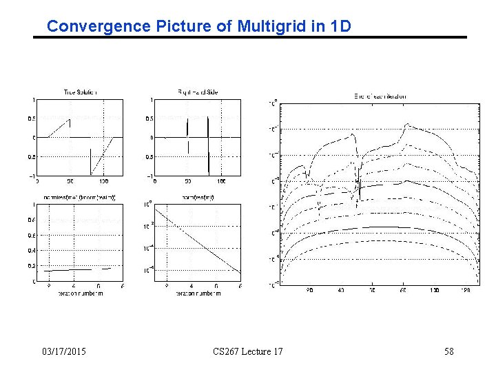
Convergence Picture of Multigrid in 1 D 03/17/2015 CS 267 Lecture 17 58

Convergence Picture of Multigrid in 2 D 03/17/2015 CS 267 Lecture 17 59

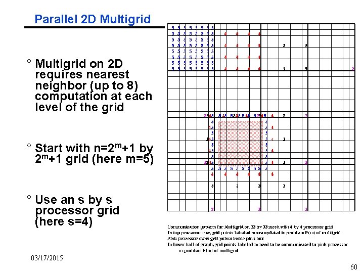
Parallel 2 D Multigrid ° Multigrid on 2 D requires nearest neighbor (up to 8) computation at each level of the grid ° Start with n=2 m+1 by 2 m+1 grid (here m=5) ° Use an s by s processor grid (here s=4) 03/17/2015 60

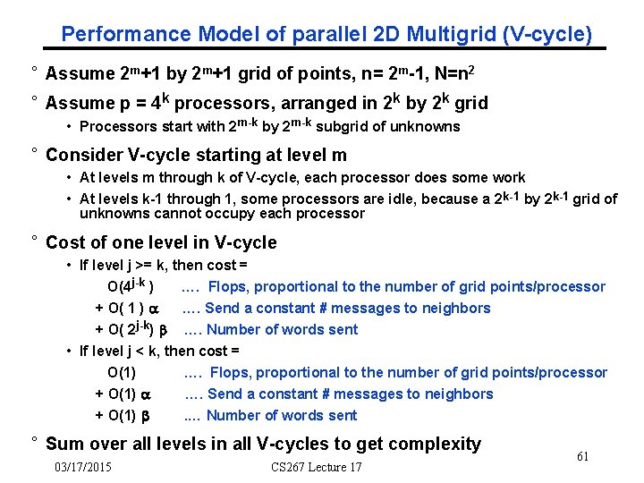
Performance Model of parallel 2 D Multigrid (V-cycle) ° Assume 2 m+1 by 2 m+1 grid of points, n= 2 m-1, N=n 2 ° Assume p = 4 k processors, arranged in 2 k by 2 k grid • Processors start with 2 m-k by 2 m-k subgrid of unknowns ° Consider V-cycle starting at level m • At levels m through k of V-cycle, each processor does some work • At levels k-1 through 1, some processors are idle, because a 2 k-1 by 2 k-1 grid of unknowns cannot occupy each processor ° Cost of one level in V-cycle • If level j >= k, then cost = O(4 j-k ) …. Flops, proportional to the number of grid points/processor + O( 1 ) a …. Send a constant # messages to neighbors + O( 2 j-k) b …. Number of words sent • If level j < k, then cost = O(1) …. Flops, proportional to the number of grid points/processor + O(1) a …. Send a constant # messages to neighbors + O(1) b. … Number of words sent ° Sum over all levels in all V-cycles to get complexity 03/17/2015 CS 267 Lecture 17 61

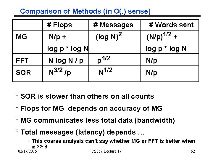
Comparison of Methods (in O(. ) sense) # Flops MG N/p + # Messages (log N)2 log p * log N # Words sent (N/p)1/2 + log p * log N FFT N log N / p p 1/2 N/p SOR N 3/2 /p N 1/2 N/p ° SOR is slower than others on all counts ° Flops for MG depends on accuracy of MG ° MG communicates less total data (bandwidth) ° Total messages (latency) depends … • This coarse analysis can’t say whether MG or FFT is better when a >> b 03/17/2015 CS 267 Lecture 17 62

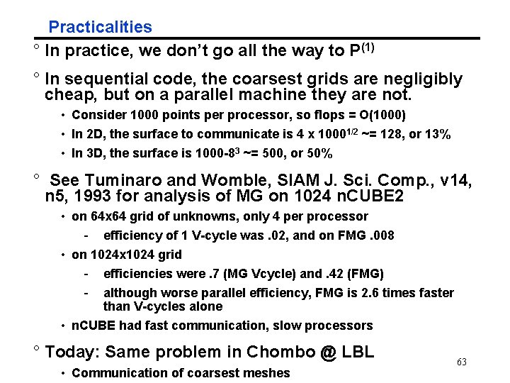
Practicalities ° In practice, we don’t go all the way to P(1) ° In sequential code, the coarsest grids are negligibly cheap, but on a parallel machine they are not. • Consider 1000 points per processor, so flops = O(1000) • In 2 D, the surface to communicate is 4 x 10001/2 ~= 128, or 13% • In 3 D, the surface is 1000 -83 ~= 500, or 50% ° See Tuminaro and Womble, SIAM J. Sci. Comp. , v 14, n 5, 1993 for analysis of MG on 1024 n. CUBE 2 • on 64 x 64 grid of unknowns, only 4 per processor - efficiency of 1 V-cycle was. 02, and on FMG. 008 • on 1024 x 1024 grid - efficiencies were. 7 (MG Vcycle) and. 42 (FMG) - although worse parallel efficiency, FMG is 2. 6 times faster than V-cycles alone • n. CUBE had fast communication, slow processors ° Today: Same problem in Chombo @ LBL • Communication of coarsest meshes 63

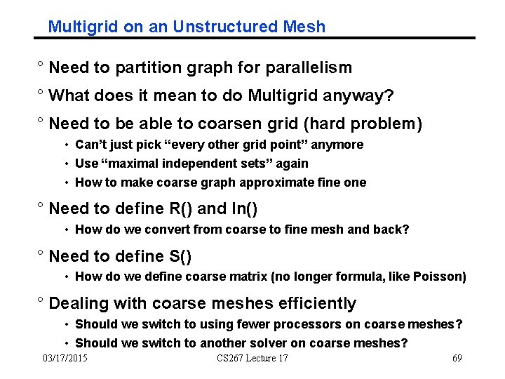
Multigrid on an Unstructured Mesh ° Need to partition graph for parallelism ° What does it mean to do Multigrid anyway? ° Need to be able to coarsen grid (hard problem) • Can’t just pick “every other grid point” anymore • Use “maximal independent sets” again • How to make coarse graph approximate fine one ° Need to define R() and In() • How do we convert from coarse to fine mesh and back? ° Need to define S() • How do we define coarse matrix (no longer formula, like Poisson) ° Dealing with coarse meshes efficiently • Should we switch to using fewer processors on coarse meshes? • Should we switch to another solver on coarse meshes? 03/17/2015 CS 267 Lecture 17 69

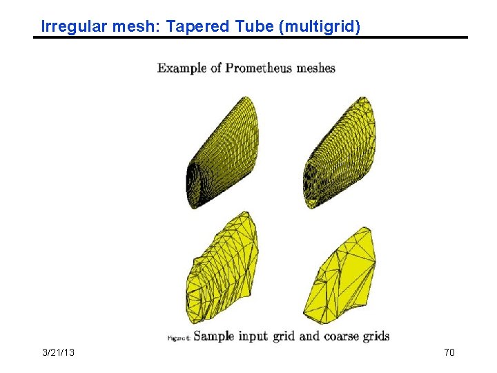
Irregular mesh: Tapered Tube (multigrid) 3/21/13 CS 267 Lecture 9 70

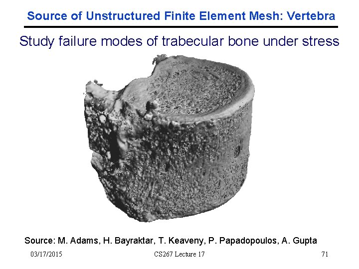
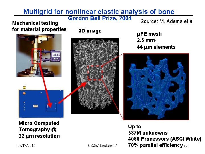
Source of Unstructured Finite Element Mesh: Vertebra Study failure modes of trabecular bone under stress Source: M. Adams, H. Bayraktar, T. Keaveny, P. Papadopoulos, A. Gupta 03/17/2015 CS 267 Lecture 17 71

Multigrid for nonlinear elastic analysis of bone Mechanical testing for material properties Gordon Bell Prize, 2004 3 D image Source: M. Adams et al m. FE mesh 2. 5 mm 3 44 mm elements Micro Computed Tomography @ 22 mm resolution 03/17/2015 CS 267 Lecture 17 Up to 537 M unknowns 4088 Processors (ASCI White) 70% parallel efficiency 72

Extra Slides

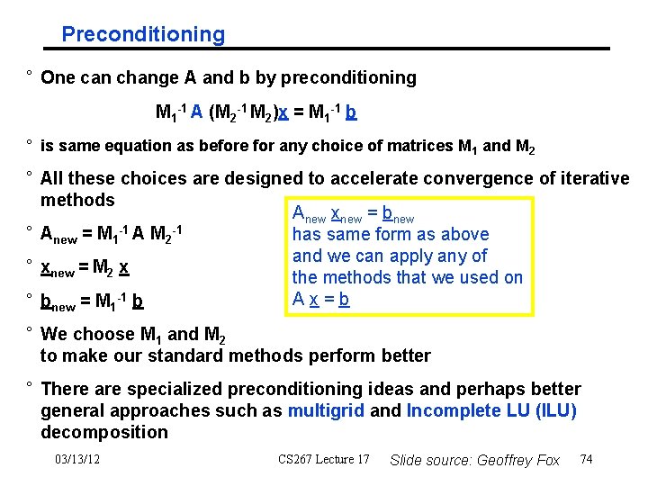
Preconditioning ° One can change A and b by preconditioning M 1 -1 A (M 2 -1 M 2)x = M 1 -1 b ° is same equation as before for any choice of matrices M 1 and M 2 ° All these choices are designed to accelerate convergence of iterative methods Anew xnew = bnew ° Anew = M 1 -1 A M 2 -1 has same form as above and we can apply any of ° xnew = M 2 x the methods that we used on Ax=b ° bnew = M 1 -1 b ° We choose M 1 and M 2 to make our standard methods perform better ° There are specialized preconditioning ideas and perhaps better general approaches such as multigrid and Incomplete LU (ILU) decomposition 03/13/12 CS 267 Lecture 17 Slide source: Geoffrey Fox 74

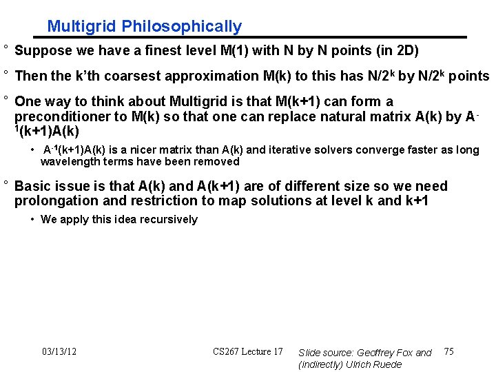
Multigrid Philosophically ° Suppose we have a finest level M(1) with N by N points (in 2 D) ° Then the k’th coarsest approximation M(k) to this has N/2 k by N/2 k points ° One way to think about Multigrid is that M(k+1) can form a preconditioner to M(k) so that one can replace natural matrix A(k) by A 1(k+1)A(k) • A-1(k+1)A(k) is a nicer matrix than A(k) and iterative solvers converge faster as long wavelength terms have been removed ° Basic issue is that A(k) and A(k+1) are of different size so we need prolongation and restriction to map solutions at level k and k+1 • We apply this idea recursively 03/13/12 CS 267 Lecture 17 Slide source: Geoffrey Fox and (indirectly) Ulrich Ruede 75

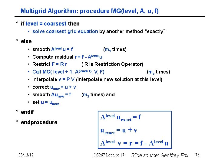
Multigrid Algorithm: procedure MG(level, A, u, f) ° if level = coarsest then • solve coarsest grid equation by another method “exactly” ° else • smooth Alevel u = f (m 1 times) • Compute residual r = f - Alevel u • Restrict F = R r ( R is Restriction Operator) • Call MG( level + 1, A(level+1), V, F) (mc times) • Interpolate v = P V (Interpolate new solution at this level) • correct unew = u + v • smooth Aunew = f (m 2 times) and • set u = unew ° endif ° endprocedure Alevel uexact = f uexact = u + v Alevel v = r = f - Alevel u 03/13/12 CS 267 Lecture 17 Slide source: Geoffrey Fox 76

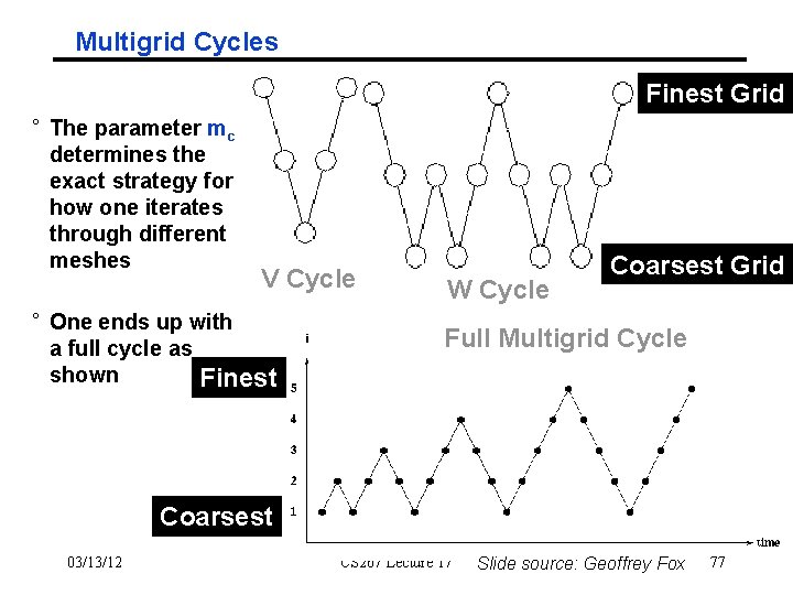
Multigrid Cycles Finest Grid ° The parameter mc determines the exact strategy for how one iterates through different meshes V Cycle ° One ends up with a full cycle as shown Finest W Cycle Coarsest Grid Full Multigrid Cycle Coarsest 03/13/12 CS 267 Lecture 17 Slide source: Geoffrey Fox 77

Extra Slides

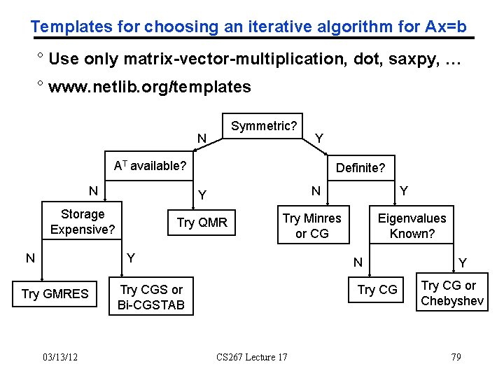
Templates for choosing an iterative algorithm for Ax=b ° Use only matrix-vector-multiplication, dot, saxpy, … ° www. netlib. org/templates Symmetric? N Y AT available? N N Y Storage Expensive? N Definite? Try QMR Try Minres or CG Y Try GMRES 03/13/12 Y Eigenvalues Known? N Try CGS or Bi-CGSTAB Try CG CS 267 Lecture 17 Y Try CG or Chebyshev 79

Summary of Jacobi, SOR and CG ° Jacobi, SOR, and CG all perform sparse-matrix-vector multiply ° For Poisson, this means nearest neighbor communication on an n-by-n grid ° It takes n = N 1/2 steps for information to travel across an n-by-n grid ° Since solution on one side of grid depends on data on other side of grid faster methods require faster ways to move information • FFT • Multigrid 03/13/12 CS 267 Lecture 17 81