CS 267 Applications of Parallel Processors Lecture 9

CS 267 Applications of Parallel Processors Lecture 9: Computational Electromagnetics Large Dense Linear Systems 2/19/97 Horst D. Simon http: //www. cs. berkeley. edu/cs 267 H. Simon - CS 267 - L 8 10/25/2020 1

Outline - Lecture 9 - Computational Electromagnetics - Sources of large dense linear systems - Review of solution of linear systems with Gaussian elimination - BLAS and memory hierarchy for linear algebra kernels H. Simon - CS 267 - L 8 10/25/2020 2

Outline - Lecture 10 - Layout of matrices on distributed memory machines - Distributed Gaussian elimination - Speeding up with advanced algorithms - LINPACK and LAPACK - LINPACK benchmark - Tflops result H. Simon - CS 267 - L 8 10/25/2020 3

Outline - Lecture 11 - Designing portable libraries for parallel machines - BLACS - Sca. LAPACK for dense linear systems - other linear algebra algorithms in Sca. LAPACK H. Simon - CS 267 - L 8 10/25/2020 4

Computational Electromagnetics - developed during 1980 s, driven by defense applications - determine the RCS (radar cross section) of airplane - reduce signature of plane (stealth technology) - other applications are antenna design, medical equipment - two fundamental numerical approaches: MOM methods of moments ( frequency domain), and finite differences (time domain) H. Simon - CS 267 - L 8 10/25/2020 5

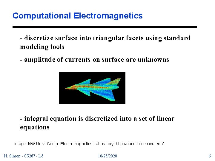
Computational Electromagnetics - discretize surface into triangular facets using standard modeling tools - amplitude of currents on surface are unknowns - integral equation is discretized into a set of linear equations image: NW Univ. Comp. Electromagnetics Laboratory http: //nueml. ece. nwu. edu/ H. Simon - CS 267 - L 8 10/25/2020 6

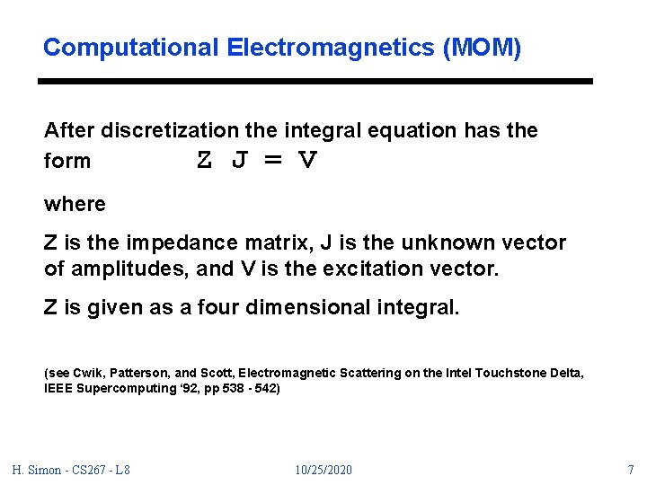
Computational Electromagnetics (MOM) After discretization the integral equation has the form Z J = V where Z is the impedance matrix, J is the unknown vector of amplitudes, and V is the excitation vector. Z is given as a four dimensional integral. (see Cwik, Patterson, and Scott, Electromagnetic Scattering on the Intel Touchstone Delta, IEEE Supercomputing ‘ 92, pp 538 - 542) H. Simon - CS 267 - L 8 10/25/2020 7

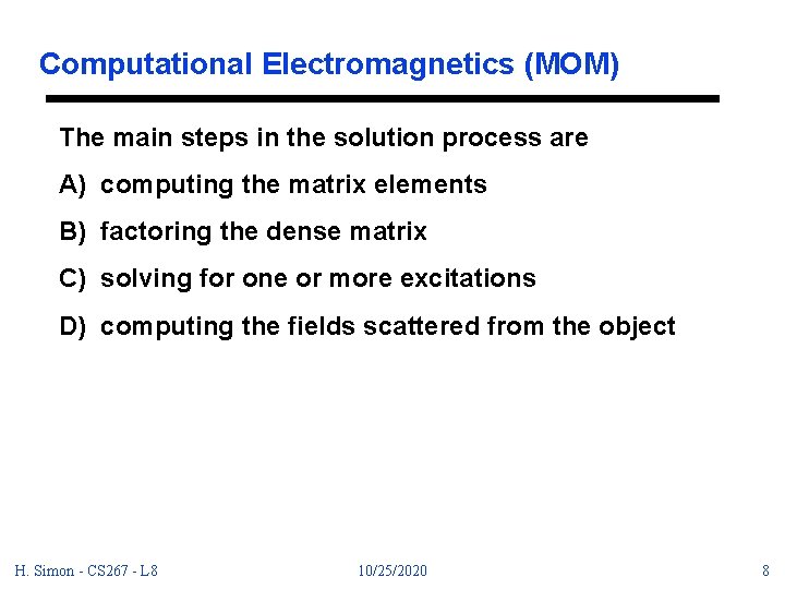
Computational Electromagnetics (MOM) The main steps in the solution process are A) computing the matrix elements B) factoring the dense matrix C) solving for one or more excitations D) computing the fields scattered from the object H. Simon - CS 267 - L 8 10/25/2020 8

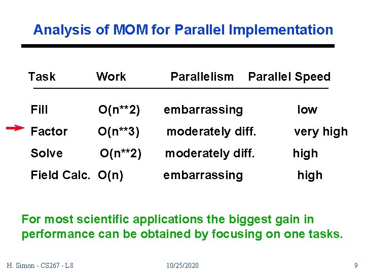
Analysis of MOM for Parallel Implementation Task Work Fill O(n**2) embarrassing low Factor O(n**3) moderately diff. very high Solve O(n**2) moderately diff. high Field Calc. O(n) Parallelism embarrassing Parallel Speed high For most scientific applications the biggest gain in performance can be obtained by focusing on one tasks. H. Simon - CS 267 - L 8 10/25/2020 9

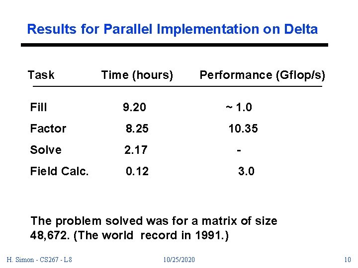
Results for Parallel Implementation on Delta Task Time (hours) Performance (Gflop/s) Fill 9. 20 ~ 1. 0 Factor 8. 25 10. 35 Solve 2. 17 - Field Calc. 0. 12 3. 0 The problem solved was for a matrix of size 48, 672. (The world record in 1991. ) H. Simon - CS 267 - L 8 10/25/2020 10

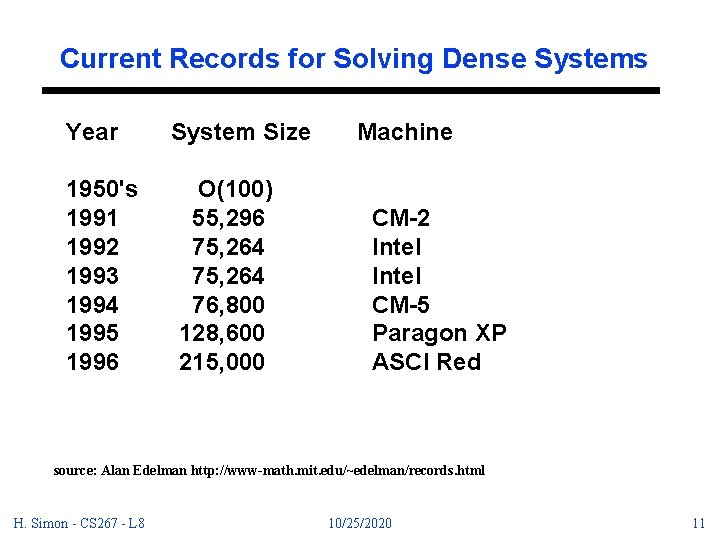
Current Records for Solving Dense Systems Year 1950's 1991 1992 1993 1994 1995 1996 System Size O(100) 55, 296 75, 264 76, 800 128, 600 215, 000 Machine CM-2 Intel CM-5 Paragon XP ASCI Red source: Alan Edelman http: //www-math. mit. edu/~edelman/records. html H. Simon - CS 267 - L 8 10/25/2020 11

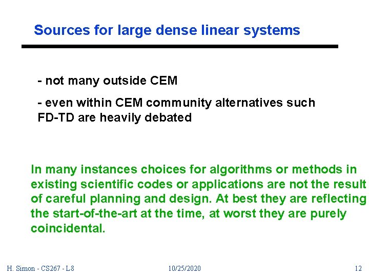
Sources for large dense linear systems - not many outside CEM - even within CEM community alternatives such FD-TD are heavily debated In many instances choices for algorithms or methods in existing scientific codes or applications are not the result of careful planning and design. At best they are reflecting the start-of-the-art at the time, at worst they are purely coincidental. H. Simon - CS 267 - L 8 10/25/2020 12

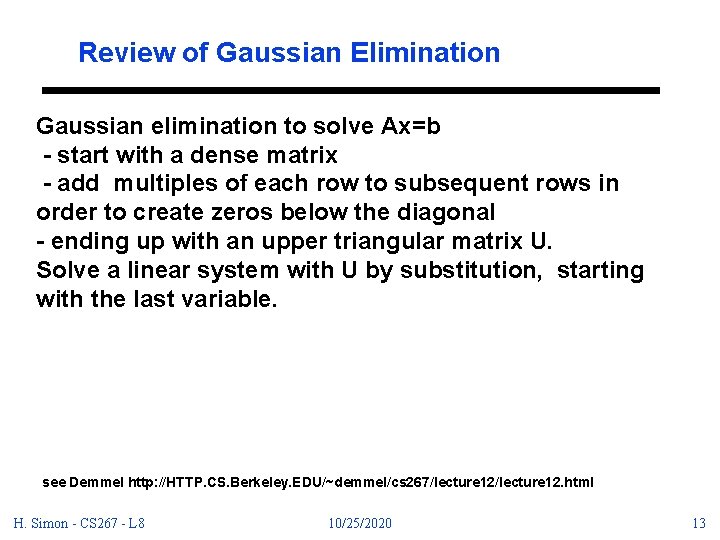
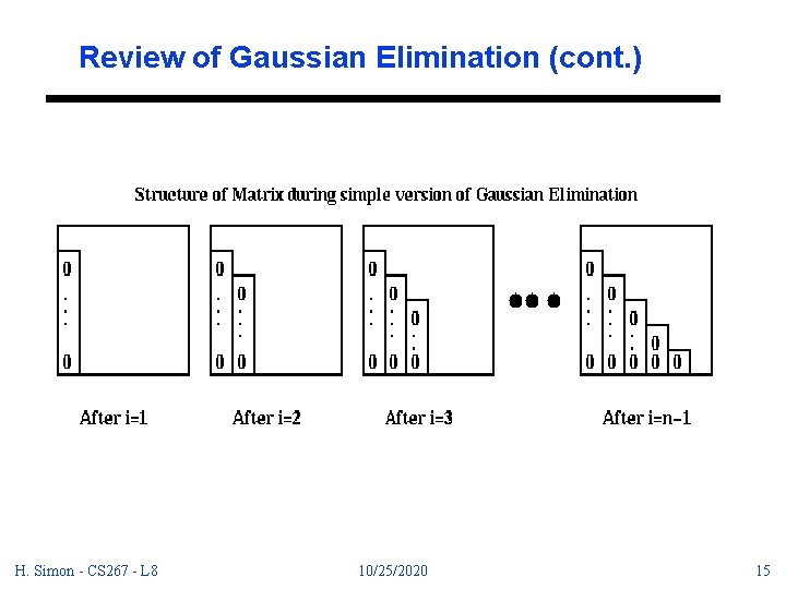
Review of Gaussian Elimination Gaussian elimination to solve Ax=b - start with a dense matrix - add multiples of each row to subsequent rows in order to create zeros below the diagonal - ending up with an upper triangular matrix U. Solve a linear system with U by substitution, starting with the last variable. see Demmel http: //HTTP. CS. Berkeley. EDU/~demmel/cs 267/lecture 12. html H. Simon - CS 267 - L 8 10/25/2020 13

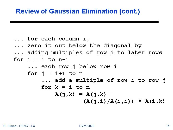
Review of Gaussian Elimination (cont. ) . . for each column i, zero it out below the diagonal by adding multiples of row i to later rows i = 1 to n-1. . . each row j below row i for j = i+1 to n. . . add a multiple of row i to row j for k = i to n A(j, k) = A(j, k) (A(j, i)/A(i, i)) * A(i, k) H. Simon - CS 267 - L 8 10/25/2020 14

Review of Gaussian Elimination (cont. ) H. Simon - CS 267 - L 8 10/25/2020 15

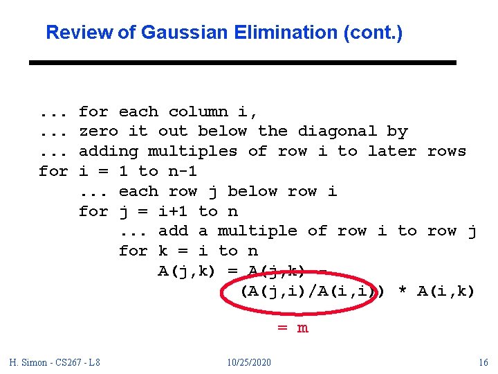
Review of Gaussian Elimination (cont. ) . . for each column i, zero it out below the diagonal by adding multiples of row i to later rows i = 1 to n-1. . . each row j below row i for j = i+1 to n. . . add a multiple of row i to row j for k = i to n A(j, k) = A(j, k) (A(j, i)/A(i, i)) * A(i, k) = m H. Simon - CS 267 - L 8 10/25/2020 16

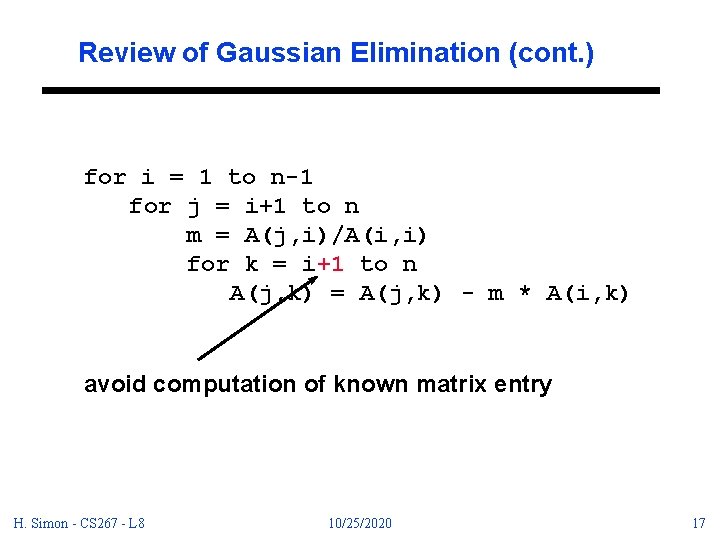
Review of Gaussian Elimination (cont. ) for i = 1 to n-1 for j = i+1 to n m = A(j, i)/A(i, i) for k = i+1 to n A(j, k) = A(j, k) - m * A(i, k) avoid computation of known matrix entry H. Simon - CS 267 - L 8 10/25/2020 17

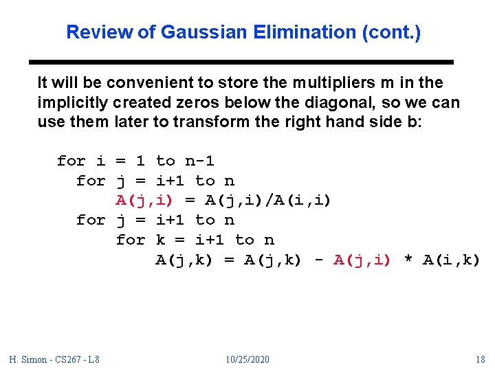
Review of Gaussian Elimination (cont. ) It will be convenient to store the multipliers m in the implicitly created zeros below the diagonal, so we can use them later to transform the right hand side b: for i = 1 to n-1 for j = i+1 to n A(j, i) = A(j, i)/A(i, i) for j = i+1 to n for k = i+1 to n A(j, k) = A(j, k) - A(j, i) * A(i, k) H. Simon - CS 267 - L 8 10/25/2020 18

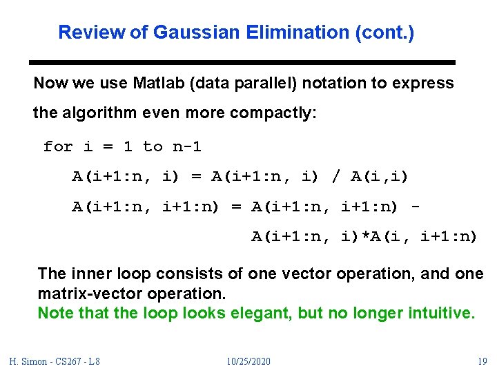
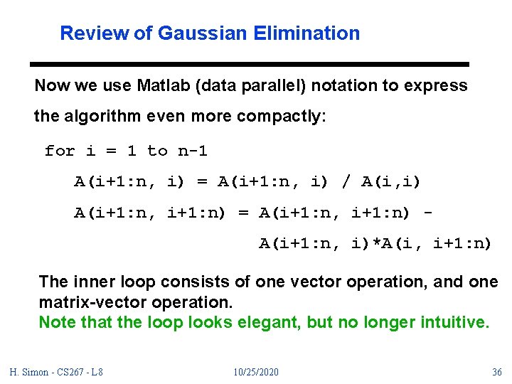
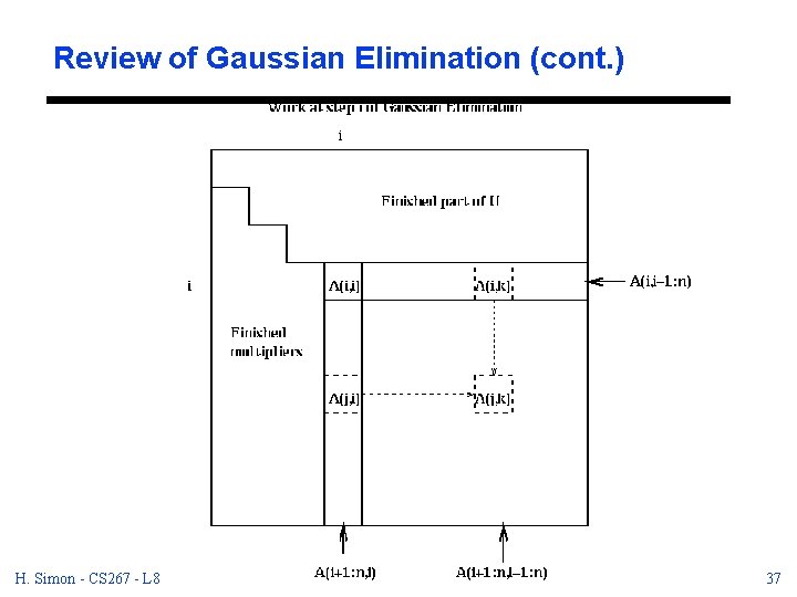
Review of Gaussian Elimination (cont. ) Now we use Matlab (data parallel) notation to express the algorithm even more compactly: for i = 1 to n-1 A(i+1: n, i) = A(i+1: n, i) / A(i, i) A(i+1: n, i+1: n) = A(i+1: n, i+1: n) A(i+1: n, i)*A(i, i+1: n) The inner loop consists of one vector operation, and one matrix-vector operation. Note that the loop looks elegant, but no longer intuitive. H. Simon - CS 267 - L 8 10/25/2020 19

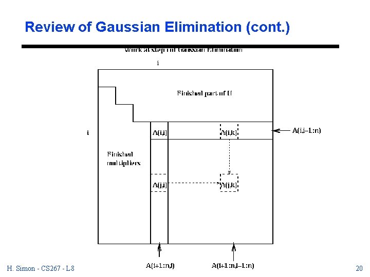
Review of Gaussian Elimination (cont. ) H. Simon - CS 267 - L 8 10/25/2020 20

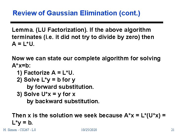
Review of Gaussian Elimination (cont. ) Lemma. (LU Factorization). If the above algorithm terminates (i. e. it did not try to divide by zero) then A = L*U. Now we can state our complete algorithm for solving A*x=b: 1) Factorize A = L*U. 2) Solve L*y = b for y by forward substitution. 3) Solve U*x = y for x by backward substitution. Then x is the solution we seek because A*x = L*(U*x) = L*y = b. H. Simon - CS 267 - L 8 10/25/2020 21

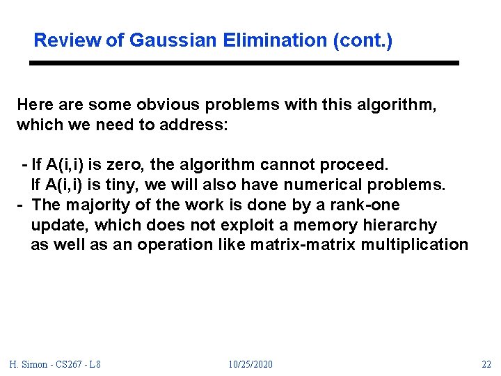
Review of Gaussian Elimination (cont. ) Here are some obvious problems with this algorithm, which we need to address: - If A(i, i) is zero, the algorithm cannot proceed. If A(i, i) is tiny, we will also have numerical problems. - The majority of the work is done by a rank-one update, which does not exploit a memory hierarchy as well as an operation like matrix-matrix multiplication H. Simon - CS 267 - L 8 10/25/2020 22

Pivoting for Small A(i, i) Why pivoting is needed? A= [ 0 1 ] [ 1 0 ] Even if A(i, i) is tiny, but not zero difficulties can arise (see example in Jim Demmel’s lecture notes). This problem is resolved by partial pivoting. H. Simon - CS 267 - L 8 10/25/2020 23

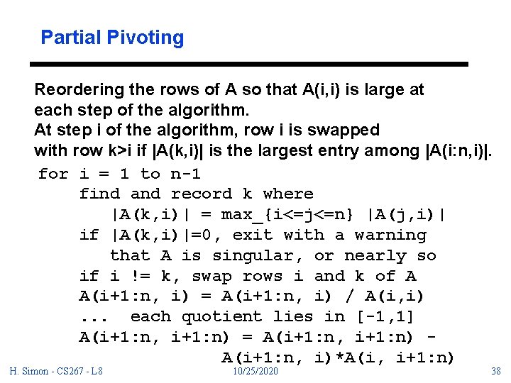
Partial Pivoting Reordering the rows of A so that A(i, i) is large at each step of the algorithm. At step i of the algorithm, row i is swapped with row k>i if |A(k, i)| is the largest entry among |A(i: n, i)|. for i = 1 to n-1 find and record k where |A(k, i)| = max_{i<=j<=n} |A(j, i)| if |A(k, i)|=0, exit with a warning that A is singular, or nearly so if i != k, swap rows i and k of A A(i+1: n, i) = A(i+1: n, i) / A(i, i). . . each quotient lies in [-1, 1] A(i+1: n, i+1: n) = A(i+1: n, i+1: n) A(i+1: n, i)*A(i, i+1: n) H. Simon - CS 267 - L 8 10/25/2020 24

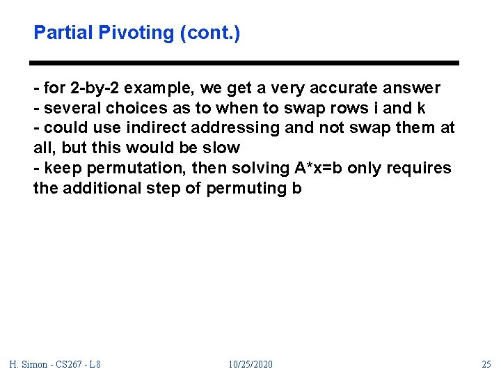
Partial Pivoting (cont. ) - for 2 -by-2 example, we get a very accurate answer - several choices as to when to swap rows i and k - could use indirect addressing and not swap them at all, but this would be slow - keep permutation, then solving A*x=b only requires the additional step of permuting b H. Simon - CS 267 - L 8 10/25/2020 25

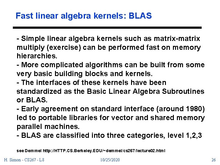
Fast linear algebra kernels: BLAS - Simple linear algebra kernels such as matrix-matrix multiply (exercise) can be performed fast on memory hierarchies. - More complicated algorithms can be built from some very basic building blocks and kernels. - The interfaces of these kernels have been standardized as the Basic Linear Algebra Subroutines or BLAS. - Early agreement on standard interface (around 1980) led to portable libraries for vector and shared memory parallel machines. - BLAS are classified into three categories, level 1, 2, 3 see Demmel http: //HTTP. CS. Berkeley. EDU/~demmel/cs 267/lecture 02. html H. Simon - CS 267 - L 8 10/25/2020 26

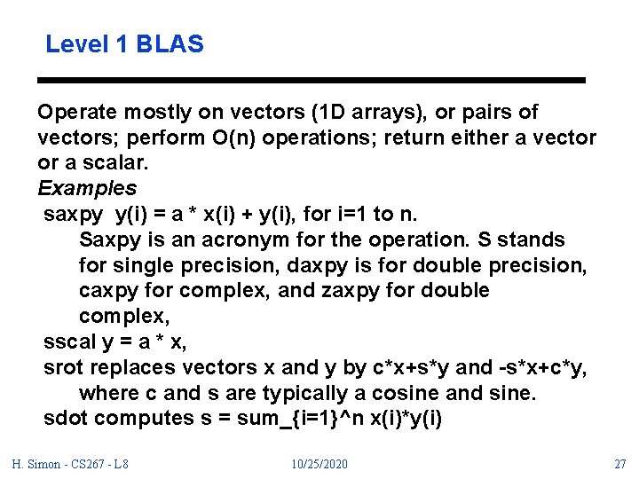
Level 1 BLAS Operate mostly on vectors (1 D arrays), or pairs of vectors; perform O(n) operations; return either a vector or a scalar. Examples saxpy y(i) = a * x(i) + y(i), for i=1 to n. Saxpy is an acronym for the operation. S stands for single precision, daxpy is for double precision, caxpy for complex, and zaxpy for double complex, sscal y = a * x, srot replaces vectors x and y by c*x+s*y and -s*x+c*y, where c and s are typically a cosine and sine. sdot computes s = sum_{i=1}^n x(i)*y(i) H. Simon - CS 267 - L 8 10/25/2020 27

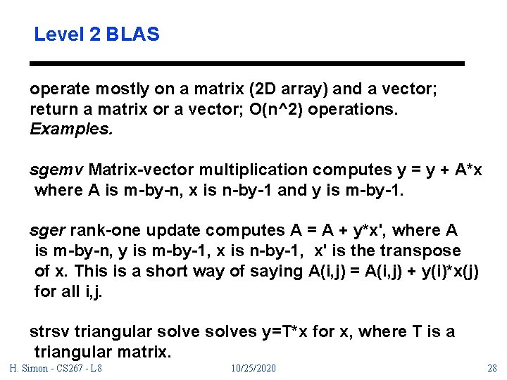
Level 2 BLAS operate mostly on a matrix (2 D array) and a vector; return a matrix or a vector; O(n^2) operations. Examples. sgemv Matrix-vector multiplication computes y = y + A*x where A is m-by-n, x is n-by-1 and y is m-by-1. sger rank-one update computes A = A + y*x', where A is m-by-n, y is m-by-1, x is n-by-1, x' is the transpose of x. This is a short way of saying A(i, j) = A(i, j) + y(i)*x(j) for all i, j. strsv triangular solves y=T*x for x, where T is a triangular matrix. H. Simon - CS 267 - L 8 10/25/2020 28

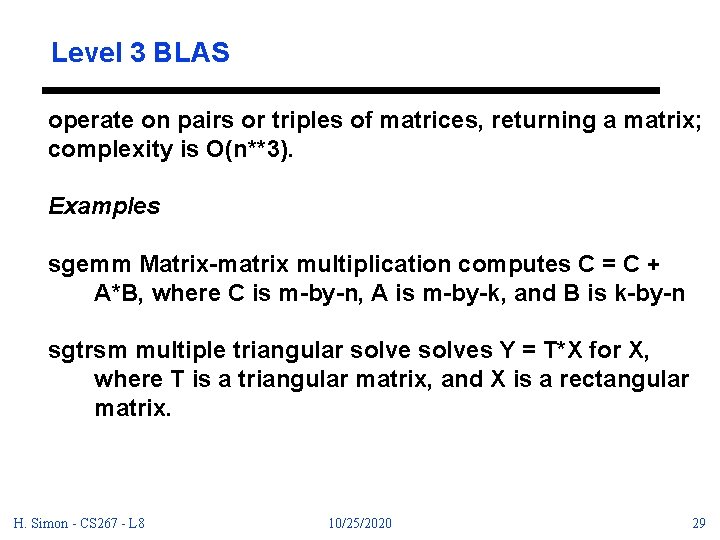
Level 3 BLAS operate on pairs or triples of matrices, returning a matrix; complexity is O(n**3). Examples sgemm Matrix-matrix multiplication computes C = C + A*B, where C is m-by-n, A is m-by-k, and B is k-by-n sgtrsm multiple triangular solves Y = T*X for X, where T is a triangular matrix, and X is a rectangular matrix. H. Simon - CS 267 - L 8 10/25/2020 29

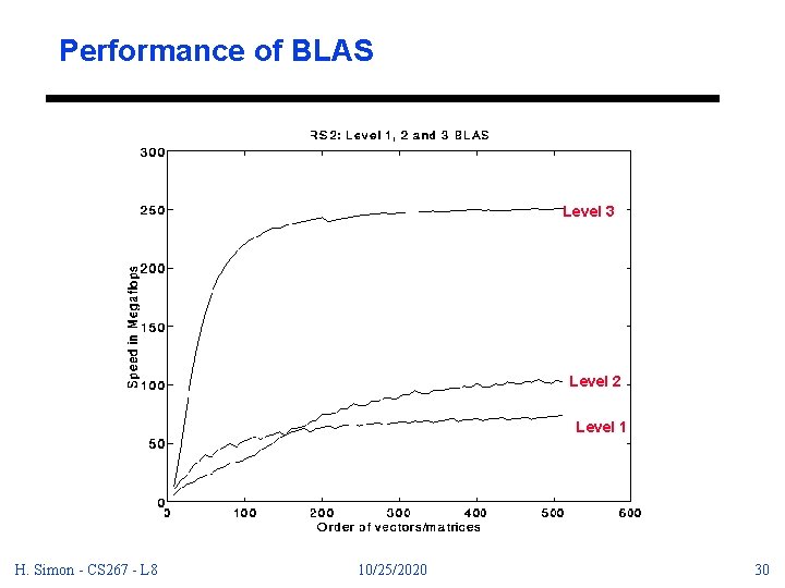
Performance of BLAS Level 3 Level 2 Level 1 H. Simon - CS 267 - L 8 10/25/2020 30

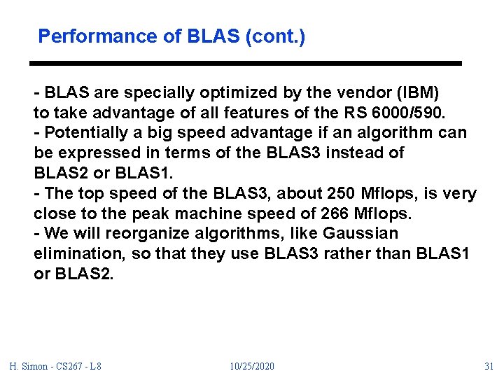
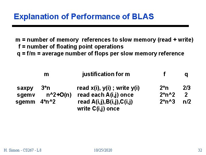
Performance of BLAS (cont. ) - BLAS are specially optimized by the vendor (IBM) to take advantage of all features of the RS 6000/590. - Potentially a big speed advantage if an algorithm can be expressed in terms of the BLAS 3 instead of BLAS 2 or BLAS 1. - The top speed of the BLAS 3, about 250 Mflops, is very close to the peak machine speed of 266 Mflops. - We will reorganize algorithms, like Gaussian elimination, so that they use BLAS 3 rather than BLAS 1 or BLAS 2. H. Simon - CS 267 - L 8 10/25/2020 31

Explanation of Performance of BLAS m = number of memory references to slow memory (read + write) f = number of floating point operations q = f/m = average number of flops per slow memory reference m justification for m saxpy 3*n read x(i), y(i) ; write y(i) sgemv n^2+O(n) read each A(i, j) once sgemm 4*n^2 read A(i, j), B(i, j), C(i, j) write C(i, j) once H. Simon - CS 267 - L 8 10/25/2020 f 2*n^2 2*n^3 q 2/3 2 n/2 32

CS 267 Applications of Parallel Processors Lecture 10: Large Dense Linear Systems Distributed Implementations 2/21/97 Horst D. Simon http: //www. cs. berkeley. edu/cs 267 H. Simon - CS 267 - L 8 10/25/2020 33

Review - Lecture 9 - computational electromagnetics and linear systems - rewritten Gaussian elimination as vector and matrix -vector operation (level 2 BLAS) - discussed the efficiency of level 3 BLAS in terms of reducing number of memory accesses H. Simon - CS 267 - L 8 10/25/2020 34

Outline - Lecture 10 - Layout of matrices on distributed memory machines - Distributed Gaussian elimination - Speeding up with advanced algorithms - LINPACK and LAPACK - LINPACK benchmark - Tflops result H. Simon - CS 267 - L 8 10/25/2020 35

Review of Gaussian Elimination Now we use Matlab (data parallel) notation to express the algorithm even more compactly: for i = 1 to n-1 A(i+1: n, i) = A(i+1: n, i) / A(i, i) A(i+1: n, i+1: n) = A(i+1: n, i+1: n) A(i+1: n, i)*A(i, i+1: n) The inner loop consists of one vector operation, and one matrix-vector operation. Note that the loop looks elegant, but no longer intuitive. H. Simon - CS 267 - L 8 10/25/2020 36

Review of Gaussian Elimination (cont. ) H. Simon - CS 267 - L 8 10/25/2020 37

Partial Pivoting Reordering the rows of A so that A(i, i) is large at each step of the algorithm. At step i of the algorithm, row i is swapped with row k>i if |A(k, i)| is the largest entry among |A(i: n, i)|. for i = 1 to n-1 find and record k where |A(k, i)| = max_{i<=j<=n} |A(j, i)| if |A(k, i)|=0, exit with a warning that A is singular, or nearly so if i != k, swap rows i and k of A A(i+1: n, i) = A(i+1: n, i) / A(i, i). . . each quotient lies in [-1, 1] A(i+1: n, i+1: n) = A(i+1: n, i+1: n) A(i+1: n, i)*A(i, i+1: n) H. Simon - CS 267 - L 8 10/25/2020 38

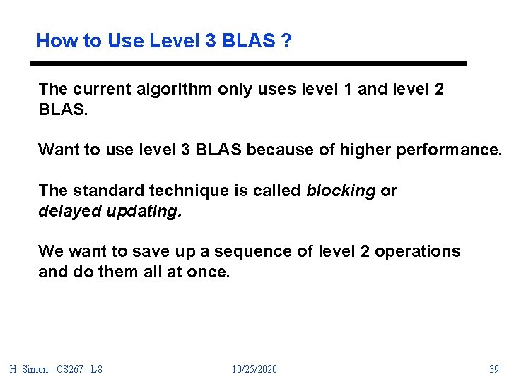
How to Use Level 3 BLAS ? The current algorithm only uses level 1 and level 2 BLAS. Want to use level 3 BLAS because of higher performance. The standard technique is called blocking or delayed updating. We want to save up a sequence of level 2 operations and do them all at once. H. Simon - CS 267 - L 8 10/25/2020 39

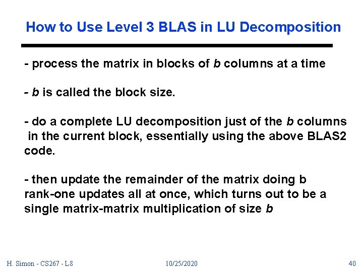
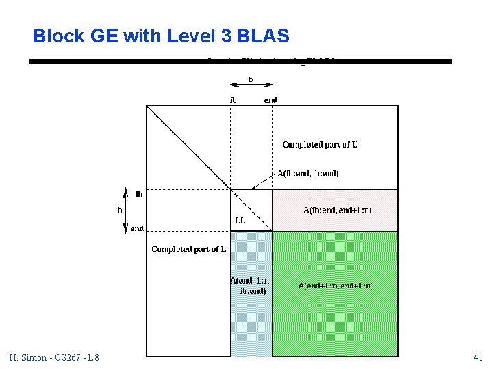
How to Use Level 3 BLAS in LU Decomposition - process the matrix in blocks of b columns at a time - b is called the block size. - do a complete LU decomposition just of the b columns in the current block, essentially using the above BLAS 2 code. - then update the remainder of the matrix doing b rank-one updates all at once, which turns out to be a single matrix-matrix multiplication of size b H. Simon - CS 267 - L 8 10/25/2020 40

Block GE with Level 3 BLAS H. Simon - CS 267 - L 8 10/25/2020 41

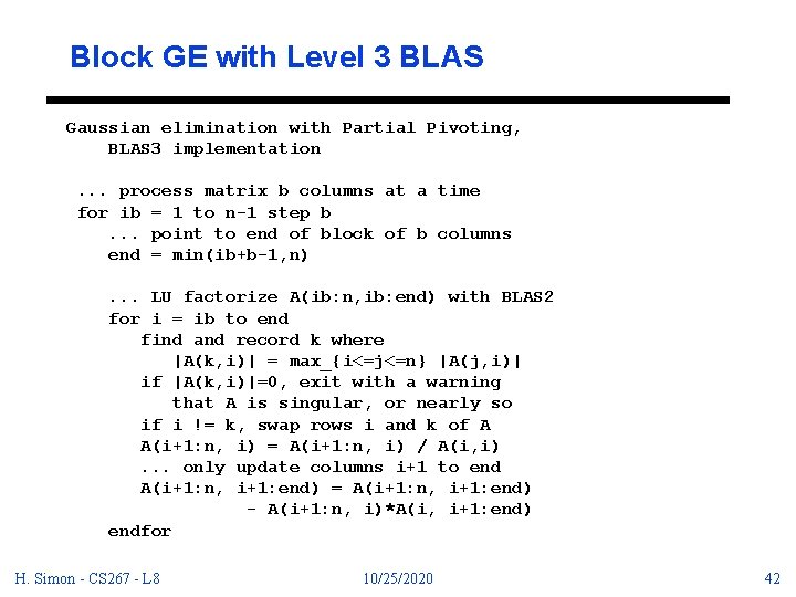
Block GE with Level 3 BLAS Gaussian elimination with Partial Pivoting, BLAS 3 implementation. . . process matrix b columns at a time for ib = 1 to n-1 step b. . . point to end of block of b columns end = min(ib+b-1, n). . . LU factorize A(ib: n, ib: end) with BLAS 2 for i = ib to end find and record k where |A(k, i)| = max_{i<=j<=n} |A(j, i)| if |A(k, i)|=0, exit with a warning that A is singular, or nearly so if i != k, swap rows i and k of A A(i+1: n, i) = A(i+1: n, i) / A(i, i). . . only update columns i+1 to end A(i+1: n, i+1: end) = A(i+1: n, i+1: end) - A(i+1: n, i)*A(i, i+1: end) endfor H. Simon - CS 267 - L 8 10/25/2020 42

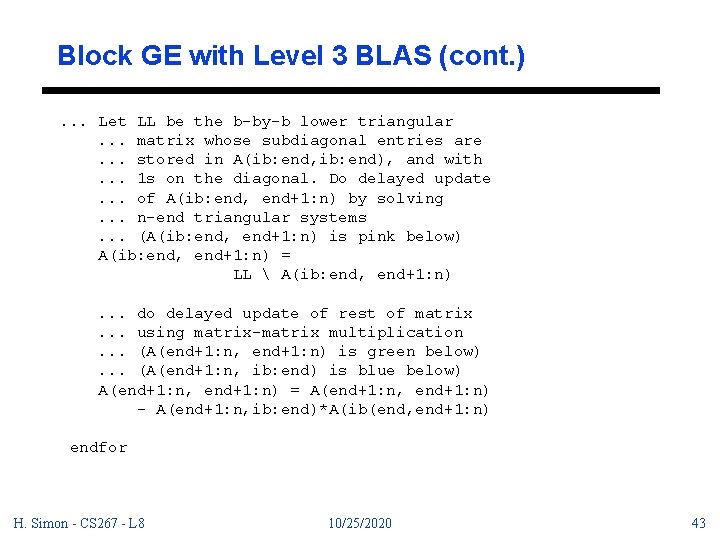
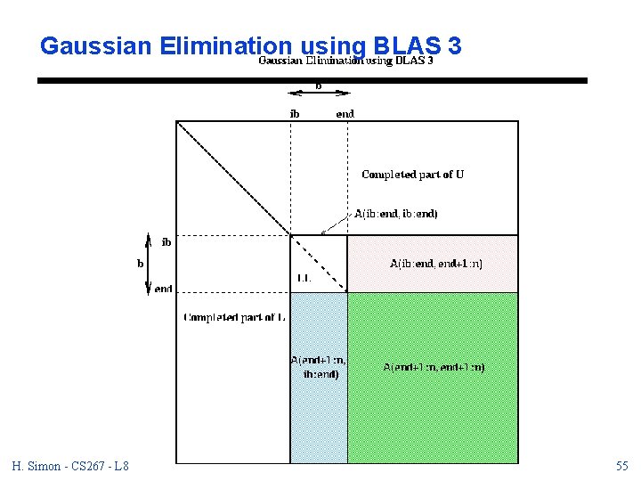
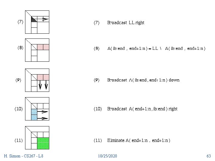
Block GE with Level 3 BLAS (cont. ). . . Let LL be the b-by-b lower triangular. . . matrix whose subdiagonal entries are. . . stored in A(ib: end, ib: end), and with. . . 1 s on the diagonal. Do delayed update. . . of A(ib: end, end+1: n) by solving. . . n-end triangular systems. . . (A(ib: end, end+1: n) is pink below) A(ib: end, end+1: n) = LL A(ib: end, end+1: n). . . do delayed update of rest of matrix. . . using matrix-matrix multiplication. . . (A(end+1: n, end+1: n) is green below). . . (A(end+1: n, ib: end) is blue below) A(end+1: n, end+1: n) = A(end+1: n, end+1: n) - A(end+1: n, ib: end)*A(ib(end, end+1: n) endfor H. Simon - CS 267 - L 8 10/25/2020 43

Block GE with Level 3 BLAS (cont. ) - LU factorization of A(ib: n, ib: end) uses the same algorithm as before (level 2 BLAS) - Solving a system of n-end equations with triangular coefficient matrix LL is a single call to a BLAS 3 subroutine (strsm) designed for that purpose. - No work or data motion is required to refer to LL; done with a pointer. - When n>>b, almost all the work is done in the final line, which multiplies an (n-end)-by-b matrix times a b-by-(n-end) matrix in a single BLAS 3 call (to sgemm). H. Simon - CS 267 - L 8 10/25/2020 44

How to select b? b will be chosen in a machine dependent way to maximize performance. A good value of b will have the following properties: - b is small enough so that the b columns currently being LU-factorized fit in the fast memory (cache, say) of the machine. - b is large enough to make matrix-matrix multiplication fast. H. Simon - CS 267 - L 8 10/25/2020 45

LINPACK - LAPACK -Sca. LAPACK LINPACK - linear systems, least squares problems level 1 BLAS - late 70 s LAPACK - redesigned LINPACK to include eigenvalue software, level 3 BLAS for parallel and shared memory parallel machines - late 80 s Sca. LAPACK - scaleable LAPACK based on BLACS for communication, distributed memory machine - mid 90 s H. Simon - CS 267 - L 8 10/25/2020 46

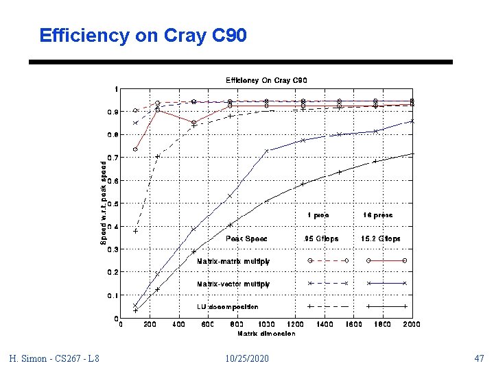
Efficiency on Cray C 90 H. Simon - CS 267 - L 8 10/25/2020 47

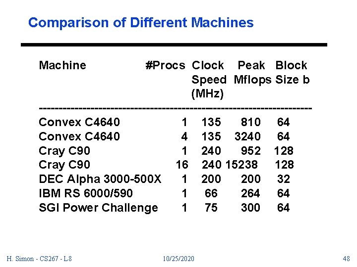
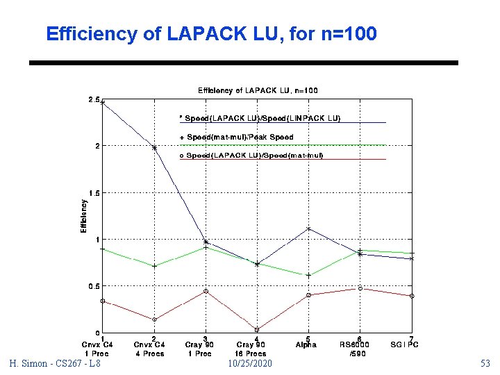
Comparison of Different Machines Machine #Procs Clock Peak Block Speed Mflops Size b (MHz) ----------------------------------Convex C 4640 1 135 810 64 Convex C 4640 4 135 3240 64 Cray C 90 1 240 952 128 Cray C 90 16 240 15238 128 DEC Alpha 3000 -500 X 1 200 32 IBM RS 6000/590 1 66 264 64 SGI Power Challenge 1 75 300 64 H. Simon - CS 267 - L 8 10/25/2020 48

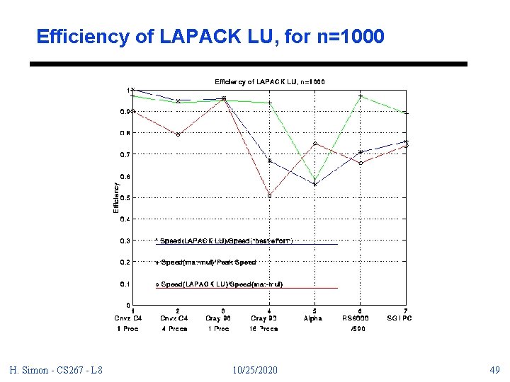
Efficiency of LAPACK LU, for n=1000 H. Simon - CS 267 - L 8 10/25/2020 49

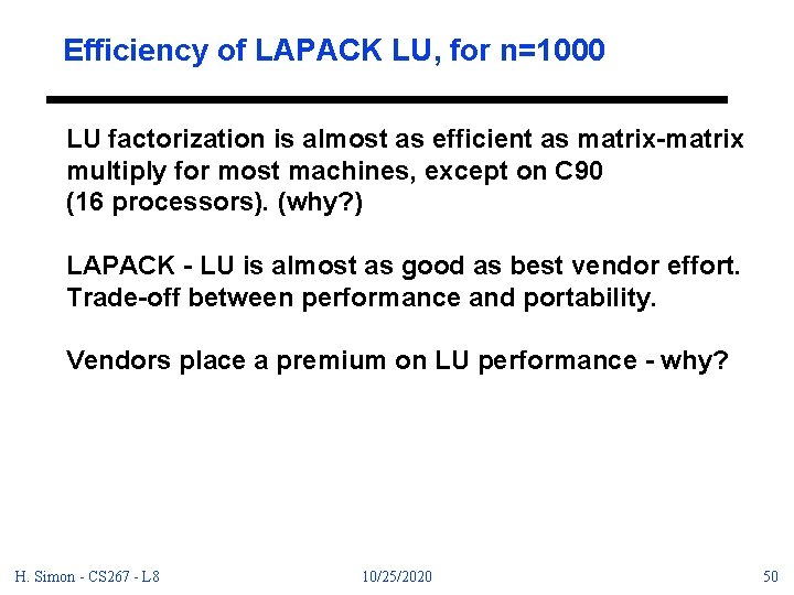
Efficiency of LAPACK LU, for n=1000 LU factorization is almost as efficient as matrix-matrix multiply for most machines, except on C 90 (16 processors). (why? ) LAPACK - LU is almost as good as best vendor effort. Trade-off between performance and portability. Vendors place a premium on LU performance - why? H. Simon - CS 267 - L 8 10/25/2020 50

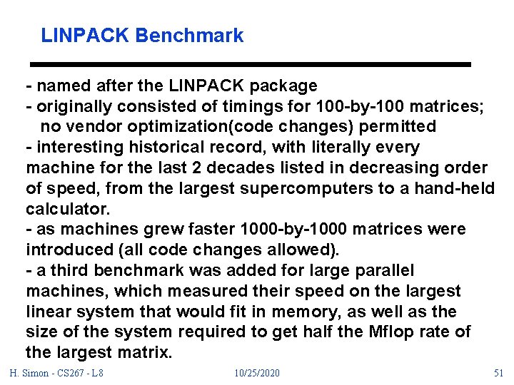
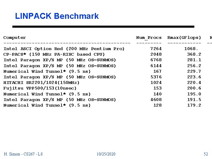
LINPACK Benchmark - named after the LINPACK package - originally consisted of timings for 100 -by-100 matrices; no vendor optimization(code changes) permitted - interesting historical record, with literally every machine for the last 2 decades listed in decreasing order of speed, from the largest supercomputers to a hand-held calculator. - as machines grew faster 1000 -by-1000 matrices were introduced (all code changes allowed). - a third benchmark was added for large parallel machines, which measured their speed on the largest linear system that would fit in memory, as well as the size of the system required to get half the Mflop rate of the largest matrix. H. Simon - CS 267 - L 8 10/25/2020 51

LINPACK Benchmark Computer ----------------------Intel ASCI Option Red (200 MHz Pentium Pro) CP-PACS* (150 MHz PA-RISC based CPU) Intel Paragon XP/S MP (50 MHz OS=SUNMOS) Numerical Wind Tunnel* (9. 5 ns) Intel Paragon XP/S MP (50 MHz OS=SUNMOS) HITACHI SR 2201/1024(150 MHz) Fujitsu VPP 500/153(10 nsec) Numerical Wind Tunnel* (9. 5 ns) Intel Paragon XP/S MP (50 MHz OS=SUNMOS) Numerical Wind Tunnel* (9. 5 ns) H. Simon - CS 267 - L 8 10/25/2020 Num_Procs ----7264 2048 6768 6144 167 5376 1024 153 140 4608 128 Rmax(GFlops) ------1068. 368. 2 281. 1 256. 2 229. 7 223. 6 220. 4 200. 6 195. 0 191. 5 179. 2 N -- 52

Efficiency of LAPACK LU, for n=100 H. Simon - CS 267 - L 8 10/25/2020 53

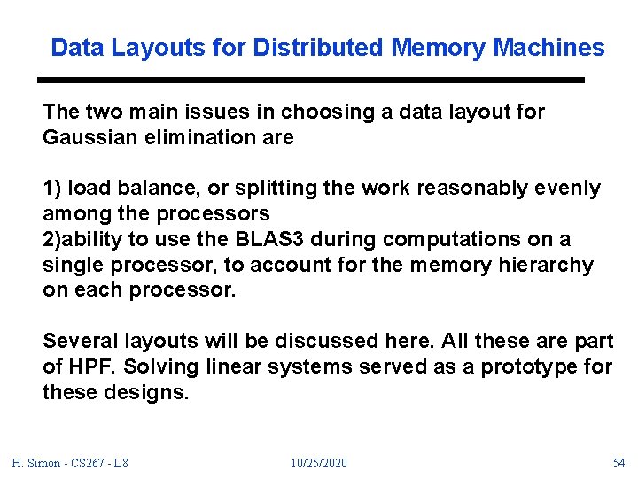
Data Layouts for Distributed Memory Machines The two main issues in choosing a data layout for Gaussian elimination are 1) load balance, or splitting the work reasonably evenly among the processors 2)ability to use the BLAS 3 during computations on a single processor, to account for the memory hierarchy on each processor. Several layouts will be discussed here. All these are part of HPF. Solving linear systems served as a prototype for these designs. H. Simon - CS 267 - L 8 10/25/2020 54

Gaussian Elimination using BLAS 3 H. Simon - CS 267 - L 8 10/25/2020 55

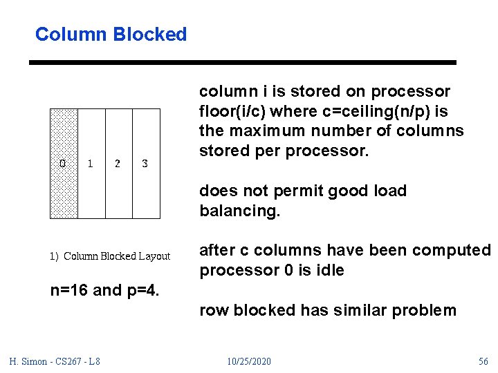
Column Blocked column i is stored on processor floor(i/c) where c=ceiling(n/p) is the maximum number of columns stored per processor. does not permit good load balancing. after c columns have been computed processor 0 is idle n=16 and p=4. row blocked has similar problem H. Simon - CS 267 - L 8 10/25/2020 56

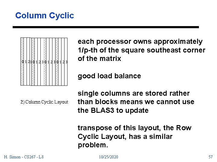
Column Cyclic each processor owns approximately 1/p-th of the square southeast corner of the matrix good load balance single columns are stored rather than blocks means we cannot use the BLAS 3 to update transpose of this layout, the Row Cyclic Layout, has a similar problem. H. Simon - CS 267 - L 8 10/25/2020 57

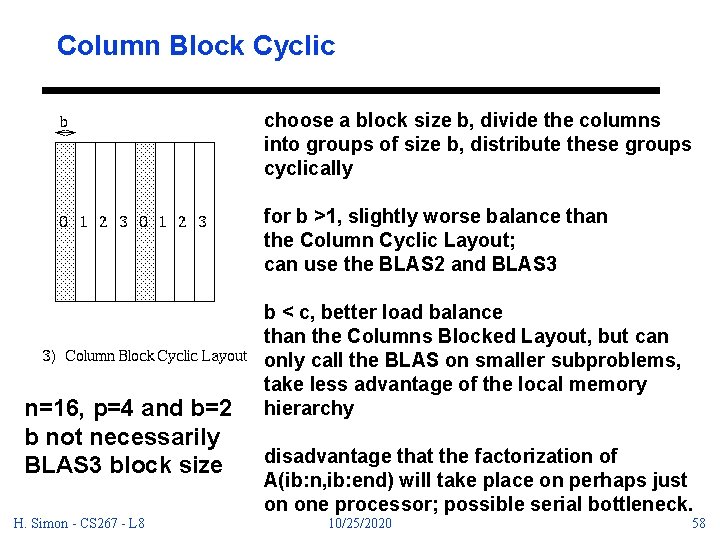
Column Block Cyclic choose a block size b, divide the columns into groups of size b, distribute these groups cyclically for b >1, slightly worse balance than the Column Cyclic Layout; can use the BLAS 2 and BLAS 3 n=16, p=4 and b=2 b not necessarily BLAS 3 block size H. Simon - CS 267 - L 8 b < c, better load balance than the Columns Blocked Layout, but can only call the BLAS on smaller subproblems, take less advantage of the local memory hierarchy disadvantage that the factorization of A(ib: n, ib: end) will take place on perhaps just on one processor; possible serial bottleneck. 10/25/2020 58

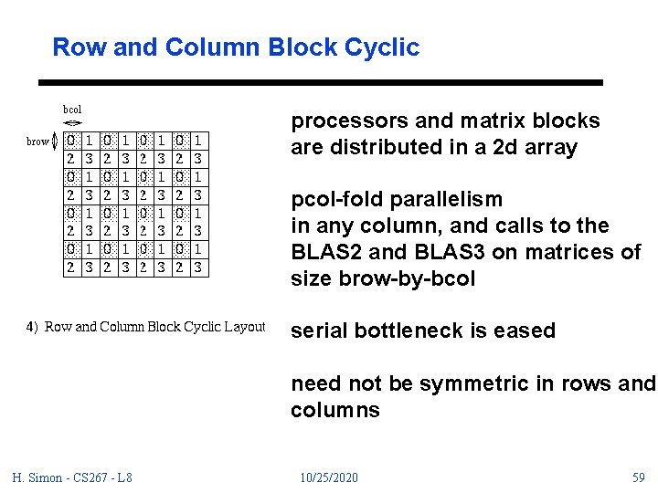
Row and Column Block Cyclic processors and matrix blocks are distributed in a 2 d array pcol-fold parallelism in any column, and calls to the BLAS 2 and BLAS 3 on matrices of size brow-by-bcol serial bottleneck is eased need not be symmetric in rows and columns H. Simon - CS 267 - L 8 10/25/2020 59

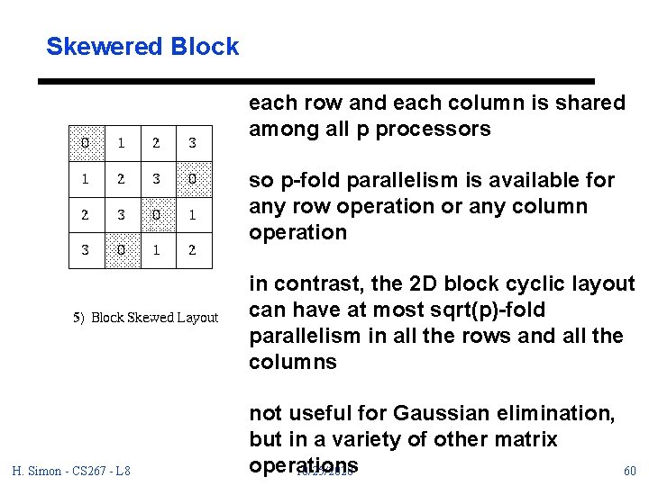
Skewered Block each row and each column is shared among all p processors so p-fold parallelism is available for any row operation or any column operation in contrast, the 2 D block cyclic layout can have at most sqrt(p)-fold parallelism in all the rows and all the columns H. Simon - CS 267 - L 8 not useful for Gaussian elimination, but in a variety of other matrix operations 10/25/2020 60

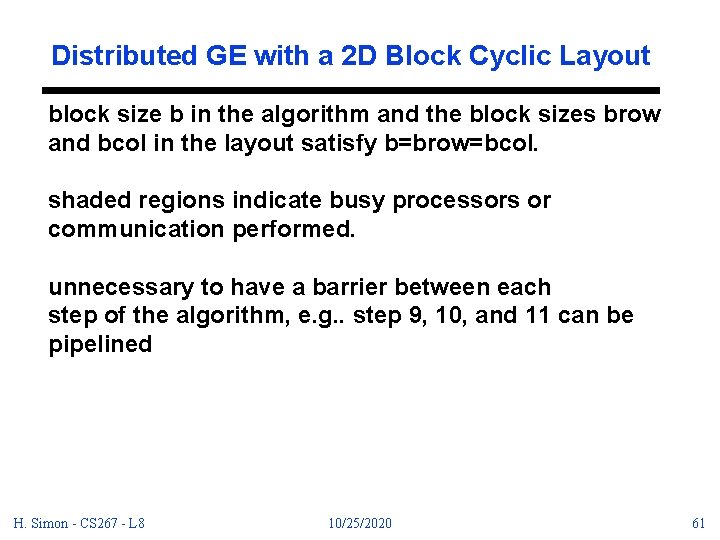
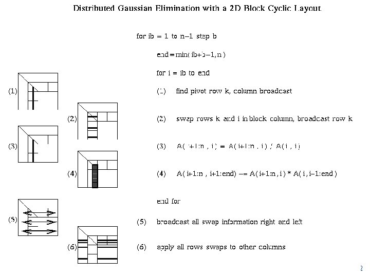
Distributed GE with a 2 D Block Cyclic Layout block size b in the algorithm and the block sizes brow and bcol in the layout satisfy b=brow=bcol. shaded regions indicate busy processors or communication performed. unnecessary to have a barrier between each step of the algorithm, e. g. . step 9, 10, and 11 can be pipelined H. Simon - CS 267 - L 8 10/25/2020 61

Distributed GE with a 2 D Block Cyclic Layout H. Simon - CS 267 - L 8 10/25/2020 62

H. Simon - CS 267 - L 8 10/25/2020 63

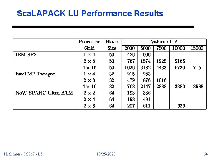
Sca. LAPACK LU Performance Results H. Simon - CS 267 - L 8 10/25/2020 64

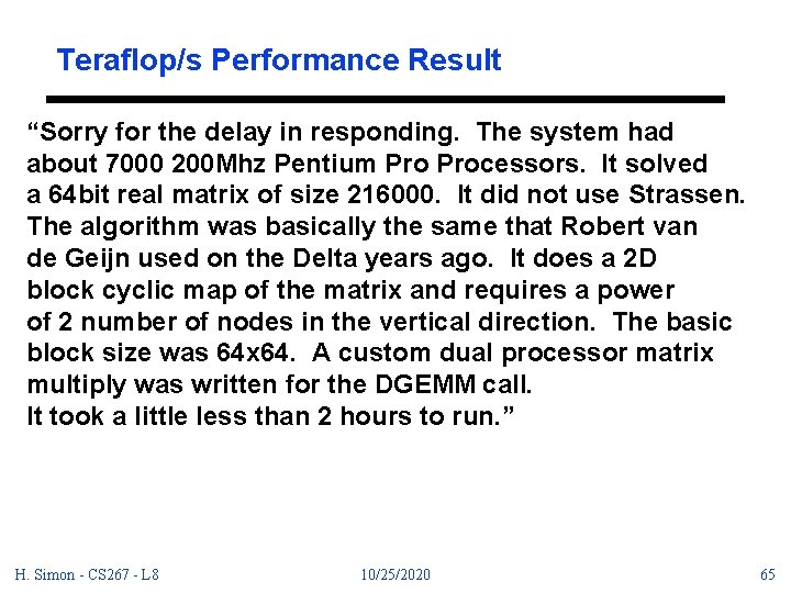
Teraflop/s Performance Result “Sorry for the delay in responding. The system had about 7000 200 Mhz Pentium Processors. It solved a 64 bit real matrix of size 216000. It did not use Strassen. The algorithm was basically the same that Robert van de Geijn used on the Delta years ago. It does a 2 D block cyclic map of the matrix and requires a power of 2 number of nodes in the vertical direction. The basic block size was 64 x 64. A custom dual processor matrix multiply was written for the DGEMM call. It took a little less than 2 hours to run. ” H. Simon - CS 267 - L 8 10/25/2020 65