Chapter 6 n Parallel Processors from Client to

Chapter 6 n Parallel Processors from Client to Cloud Chapter 6 — Parallel Processors from Client to Cloud — 1

n Goal: connecting multiple computers to get higher performance n n n High throughput for independent jobs Parallel processing program n n Multiprocessors Scalability, availability, power efficiency Task-level (process-level) parallelism n n § 6. 1 Introduction Single program run on multiple processors Multicore microprocessors n Chips with multiple processors (cores) Chapter 6 — Parallel Processors from Client to Cloud — 2

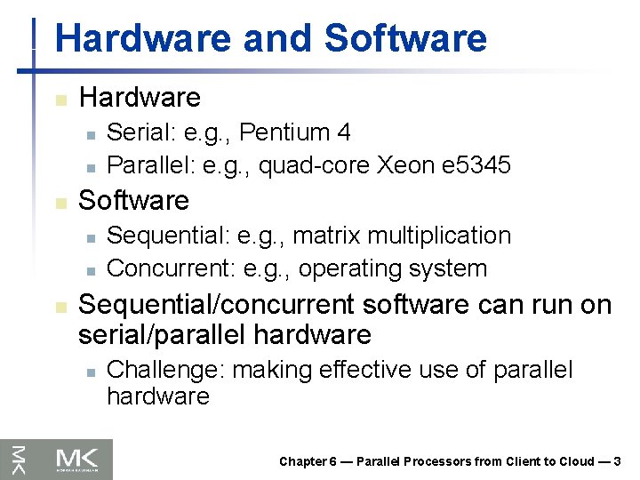
Hardware and Software n Hardware n n n Software n n n Serial: e. g. , Pentium 4 Parallel: e. g. , quad-core Xeon e 5345 Sequential: e. g. , matrix multiplication Concurrent: e. g. , operating system Sequential/concurrent software can run on serial/parallel hardware n Challenge: making effective use of parallel hardware Chapter 6 — Parallel Processors from Client to Cloud — 3

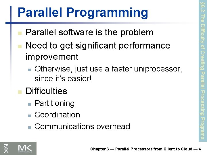
n n Parallel software is the problem Need to get significant performance improvement n n Otherwise, just use a faster uniprocessor, since it’s easier! Difficulties n n n Partitioning Coordination Communications overhead § 6. 2 The Difficulty of Creating Parallel Processing Programs Parallel Programming Chapter 6 — Parallel Processors from Client to Cloud — 4

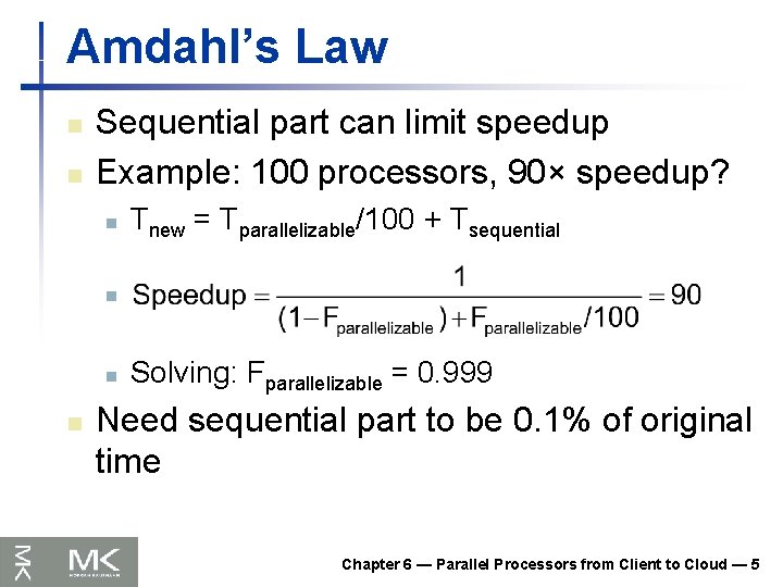
Amdahl’s Law n n Sequential part can limit speedup Example: 100 processors, 90× speedup? n Tnew = Tparallelizable/100 + Tsequential n n n Solving: Fparallelizable = 0. 999 Need sequential part to be 0. 1% of original time Chapter 6 — Parallel Processors from Client to Cloud — 5

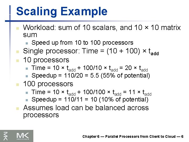
Scaling Example n Workload: sum of 10 scalars, and 10 × 10 matrix sum n n n Single processor: Time = (10 + 100) × tadd 10 processors n n n Time = 10 × tadd + 100/10 × tadd = 20 × tadd Speedup = 110/20 = 5. 5 (55% of potential) 100 processors n n n Speed up from 10 to 100 processors Time = 10 × tadd + 100/100 × tadd = 11 × tadd Speedup = 110/11 = 10 (10% of potential) Assumes load can be balanced across processors Chapter 6 — Parallel Processors from Client to Cloud — 6

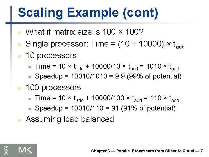
Scaling Example (cont) n n n What if matrix size is 100 × 100? Single processor: Time = (10 + 10000) × tadd 10 processors n n n 100 processors n n n Time = 10 × tadd + 10000/10 × tadd = 1010 × tadd Speedup = 10010/1010 = 9. 9 (99% of potential) Time = 10 × tadd + 10000/100 × tadd = 110 × tadd Speedup = 10010/110 = 91 (91% of potential) Assuming load balanced Chapter 6 — Parallel Processors from Client to Cloud — 7

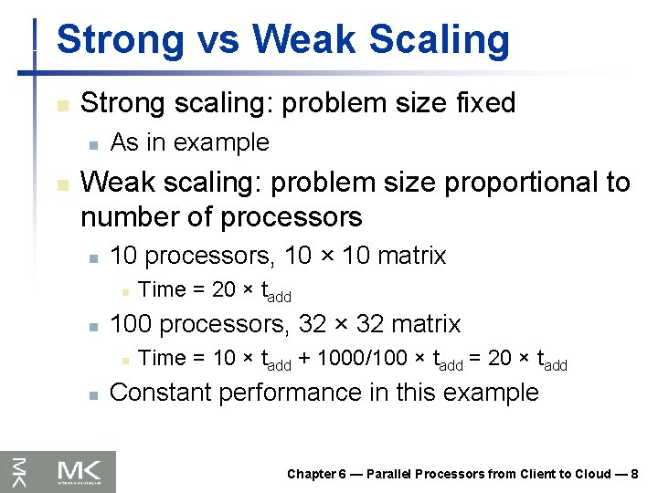
Strong vs Weak Scaling n Strong scaling: problem size fixed n n As in example Weak scaling: problem size proportional to number of processors n 10 processors, 10 × 10 matrix n n 100 processors, 32 × 32 matrix n n Time = 20 × tadd Time = 10 × tadd + 1000/100 × tadd = 20 × tadd Constant performance in this example Chapter 6 — Parallel Processors from Client to Cloud — 8

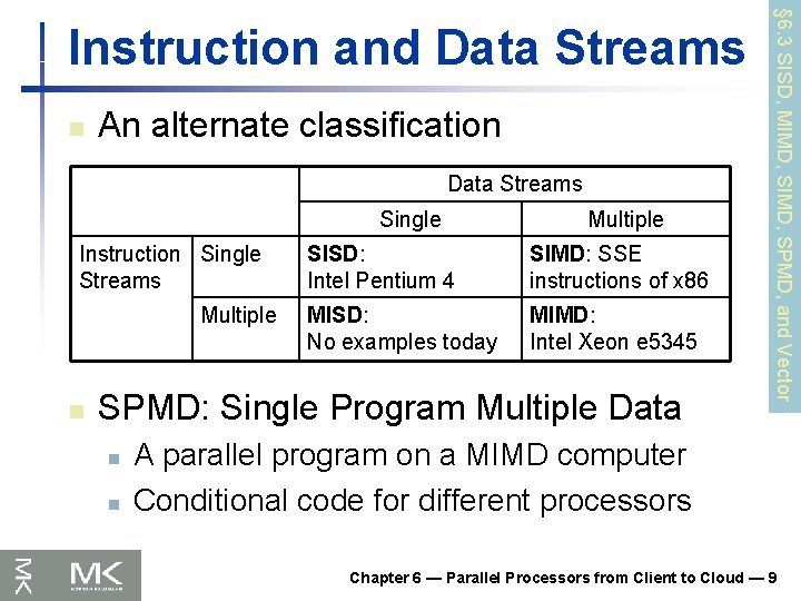
n An alternate classification Data Streams Single Instruction Single Streams Multiple n Multiple SISD: Intel Pentium 4 SIMD: SSE instructions of x 86 MISD: No examples today MIMD: Intel Xeon e 5345 SPMD: Single Program Multiple Data n n § 6. 3 SISD, MIMD, SPMD, and Vector Instruction and Data Streams A parallel program on a MIMD computer Conditional code for different processors Chapter 6 — Parallel Processors from Client to Cloud — 9

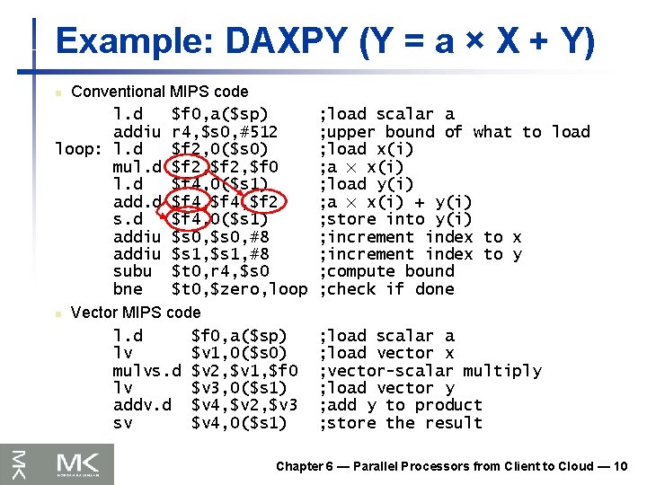
Example: DAXPY (Y = a × X + Y) Conventional MIPS code l. d $f 0, a($sp) addiu r 4, $s 0, #512 loop: l. d $f 2, 0($s 0) mul. d $f 2, $f 0 l. d $f 4, 0($s 1) add. d $f 4, $f 2 s. d $f 4, 0($s 1) addiu $s 0, #8 addiu $s 1, #8 subu $t 0, r 4, $s 0 bne $t 0, $zero, loop n Vector MIPS code l. d $f 0, a($sp) lv $v 1, 0($s 0) mulvs. d $v 2, $v 1, $f 0 lv $v 3, 0($s 1) addv. d $v 4, $v 2, $v 3 sv $v 4, 0($s 1) n ; load scalar a ; upper bound of what to load ; load x(i) ; a × x(i) ; load y(i) ; a × x(i) + y(i) ; store into y(i) ; increment index to x ; increment index to y ; compute bound ; check if done ; load scalar a ; load vector x ; vector-scalar multiply ; load vector y ; add y to product ; store the result Chapter 6 — Parallel Processors from Client to Cloud — 10

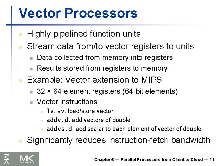
Vector Processors n n Highly pipelined function units Stream data from/to vector registers to units n n n Data collected from memory into registers Results stored from registers to memory Example: Vector extension to MIPS n n 32 × 64 -element registers (64 -bit elements) Vector instructions n n lv, sv: load/store vector addv. d: add vectors of double addvs. d: add scalar to each element of vector of double Significantly reduces instruction-fetch bandwidth Chapter 6 — Parallel Processors from Client to Cloud — 11

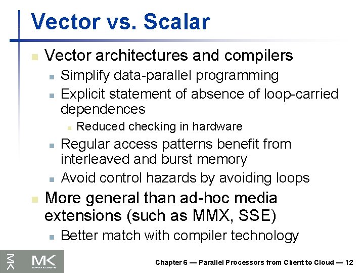
Vector vs. Scalar n Vector architectures and compilers n n Simplify data-parallel programming Explicit statement of absence of loop-carried dependences n n Reduced checking in hardware Regular access patterns benefit from interleaved and burst memory Avoid control hazards by avoiding loops More general than ad-hoc media extensions (such as MMX, SSE) n Better match with compiler technology Chapter 6 — Parallel Processors from Client to Cloud — 12

SIMD n Operate elementwise on vectors of data n E. g. , MMX and SSE instructions in x 86 n n All processors execute the same instruction at the same time n n Multiple data elements in 128 -bit wide registers Each with different data address, etc. Simplifies synchronization Reduced instruction control hardware Works best for highly data-parallel applications Chapter 6 — Parallel Processors from Client to Cloud — 13

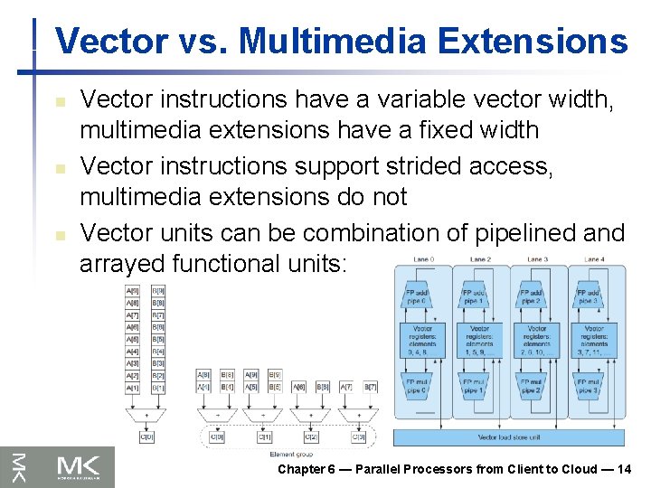
Vector vs. Multimedia Extensions n n n Vector instructions have a variable vector width, multimedia extensions have a fixed width Vector instructions support strided access, multimedia extensions do not Vector units can be combination of pipelined and arrayed functional units: Chapter 6 — Parallel Processors from Client to Cloud — 14

n Performing multiple threads of execution in parallel n n n Fine-grain multithreading n n Replicate registers, PC, etc. Fast switching between threads § 6. 4 Hardware Multithreading Switch threads after each cycle Interleave instruction execution If one thread stalls, others are executed Coarse-grain multithreading n n Only switch on long stall (e. g. , L 2 -cache miss) Simplifies hardware, but doesn’t hide short stalls (eg, data hazards) Chapter 6 — Parallel Processors from Client to Cloud — 15

Simultaneous Multithreading n In multiple-issue dynamically scheduled processor n n Schedule instructions from multiple threads Instructions from independent threads execute when function units are available Within threads, dependencies handled by scheduling and register renaming Example: Intel Pentium-4 HT n Two threads: duplicated registers, shared function units and caches Chapter 6 — Parallel Processors from Client to Cloud — 16

Future of Multithreading n n Will it survive? In what form? Power considerations simplified microarchitectures n n Tolerating cache-miss latency n n Simpler forms of multithreading Thread switch may be most effective Multiple simple cores might share resources more effectively Chapter 6 — Parallel Processors from Client to Cloud — 17

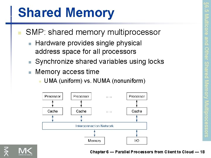
n SMP: shared memory multiprocessor n n n Hardware provides single physical address space for all processors Synchronize shared variables using locks Memory access time n UMA (uniform) vs. NUMA (nonuniform) § 6. 5 Multicore and Other Shared Memory Multiprocessors Shared Memory Chapter 6 — Parallel Processors from Client to Cloud — 18

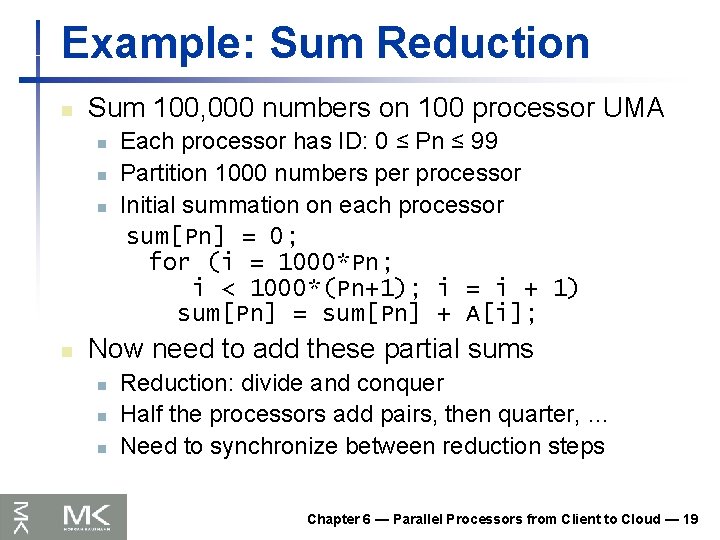
Example: Sum Reduction n Sum 100, 000 numbers on 100 processor UMA n n Each processor has ID: 0 ≤ Pn ≤ 99 Partition 1000 numbers per processor Initial summation on each processor sum[Pn] = 0; for (i = 1000*Pn; i < 1000*(Pn+1); i = i + 1) sum[Pn] = sum[Pn] + A[i]; Now need to add these partial sums n n n Reduction: divide and conquer Half the processors add pairs, then quarter, … Need to synchronize between reduction steps Chapter 6 — Parallel Processors from Client to Cloud — 19

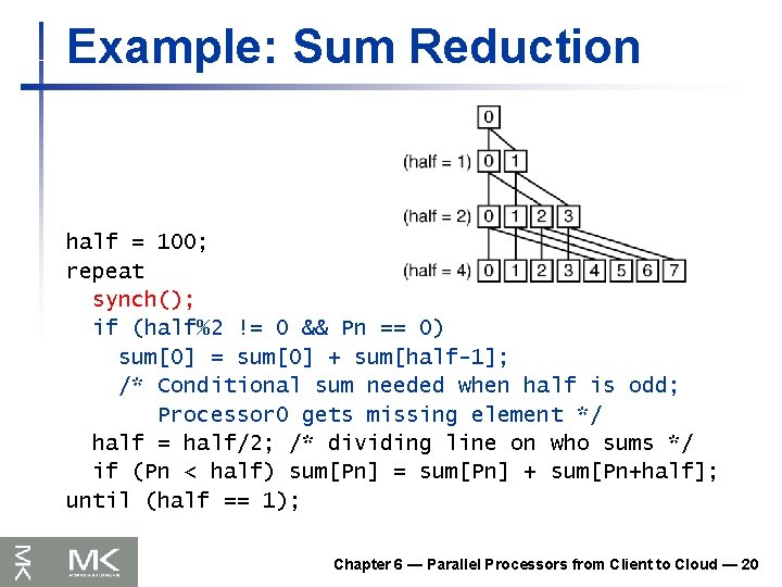
Example: Sum Reduction half = 100; repeat synch(); if (half%2 != 0 && Pn == 0) sum[0] = sum[0] + sum[half-1]; /* Conditional sum needed when half is odd; Processor 0 gets missing element */ half = half/2; /* dividing line on who sums */ if (Pn < half) sum[Pn] = sum[Pn] + sum[Pn+half]; until (half == 1); Chapter 6 — Parallel Processors from Client to Cloud — 20

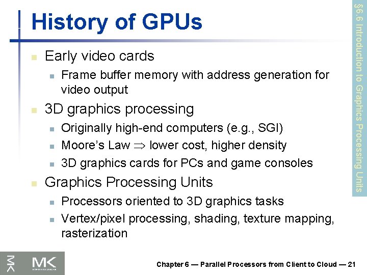
n Early video cards n n 3 D graphics processing n n Frame buffer memory with address generation for video output Originally high-end computers (e. g. , SGI) Moore’s Law lower cost, higher density 3 D graphics cards for PCs and game consoles Graphics Processing Units n n § 6. 6 Introduction to Graphics Processing Units History of GPUs Processors oriented to 3 D graphics tasks Vertex/pixel processing, shading, texture mapping, rasterization Chapter 6 — Parallel Processors from Client to Cloud — 21

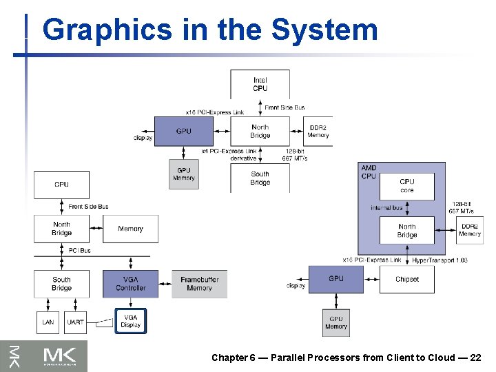
Graphics in the System Chapter 6 — Parallel Processors from Client to Cloud — 22

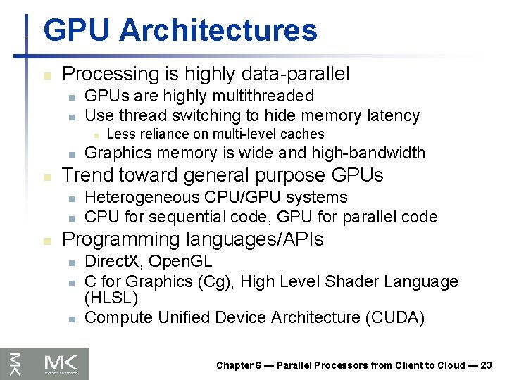
GPU Architectures n Processing is highly data-parallel n n GPUs are highly multithreaded Use thread switching to hide memory latency n n n Graphics memory is wide and high-bandwidth Trend toward general purpose GPUs n n n Less reliance on multi-level caches Heterogeneous CPU/GPU systems CPU for sequential code, GPU for parallel code Programming languages/APIs n n n Direct. X, Open. GL C for Graphics (Cg), High Level Shader Language (HLSL) Compute Unified Device Architecture (CUDA) Chapter 6 — Parallel Processors from Client to Cloud — 23

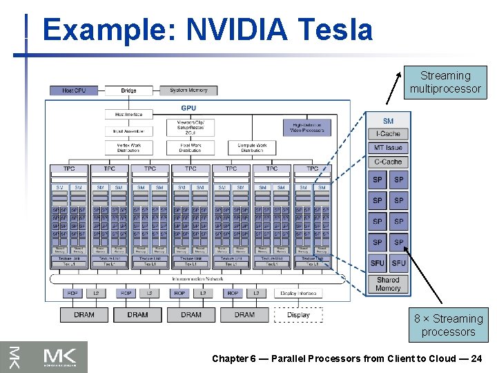
Example: NVIDIA Tesla Streaming multiprocessor 8 × Streaming processors Chapter 6 — Parallel Processors from Client to Cloud — 24

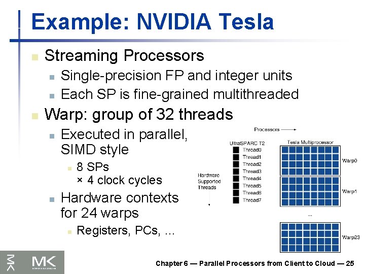
Example: NVIDIA Tesla n Streaming Processors n n n Single-precision FP and integer units Each SP is fine-grained multithreaded Warp: group of 32 threads n Executed in parallel, SIMD style n n 8 SPs × 4 clock cycles Hardware contexts for 24 warps n Registers, PCs, … Chapter 6 — Parallel Processors from Client to Cloud — 25

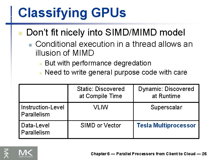
Classifying GPUs n Don’t fit nicely into SIMD/MIMD model n Conditional execution in a thread allows an illusion of MIMD n n But with performance degredation Need to write general purpose code with care Instruction-Level Parallelism Data-Level Parallelism Static: Discovered at Compile Time Dynamic: Discovered at Runtime VLIW Superscalar SIMD or Vector Tesla Multiprocessor Chapter 6 — Parallel Processors from Client to Cloud — 26

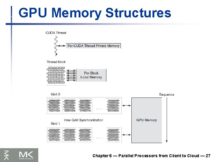
GPU Memory Structures Chapter 6 — Parallel Processors from Client to Cloud — 27

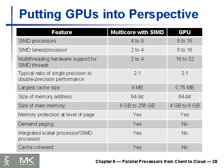
Putting GPUs into Perspective Feature Multicore with SIMD GPU SIMD processors 4 to 8 8 to 16 SIMD lanes/processor 2 to 4 8 to 16 Multithreading hardware support for SIMD threads 2 to 4 16 to 32 2: 1 Largest cache size 8 MB 0. 75 MB Size of memory address 64 -bit 8 GB to 256 GB 4 GB to 6 GB Memory protection at level of page Yes Demand paging Yes No Integrated scalar processor/SIMD processor Yes No Cache coherent Yes No Typical ratio of single precision to double-precision performance Size of main memory Chapter 6 — Parallel Processors from Client to Cloud — 28

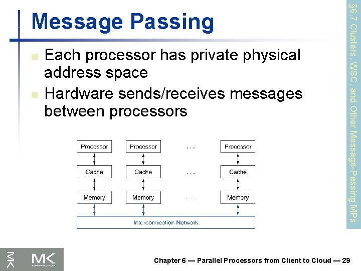
n n Each processor has private physical address space Hardware sends/receives messages between processors § 6. 7 Clusters, WSC, and Other Message-Passing MPs Message Passing Chapter 6 — Parallel Processors from Client to Cloud — 29

Loosely Coupled Clusters n Network of independent computers n n Each has private memory and OS Connected using I/O system n n Suitable for applications with independent tasks n n n E. g. , Ethernet/switch, Internet Web servers, databases, simulations, … High availability, scalable, affordable Problems n n Administration cost (prefer virtual machines) Low interconnect bandwidth n c. f. processor/memory bandwidth on an SMP Chapter 6 — Parallel Processors from Client to Cloud — 30

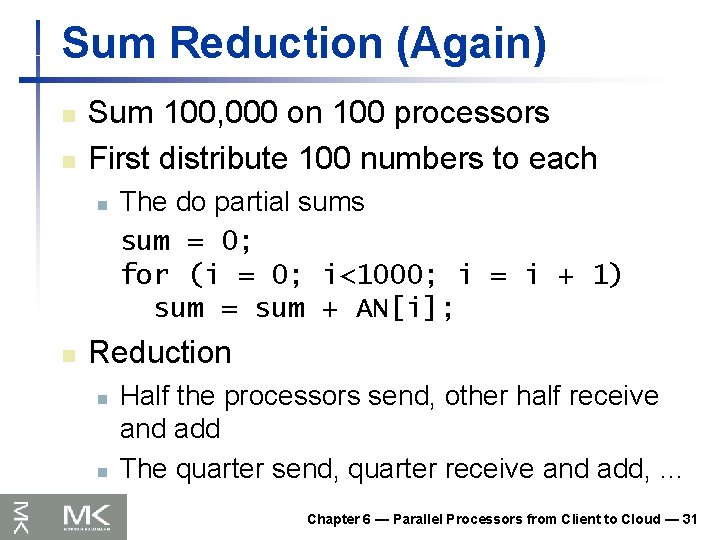
Sum Reduction (Again) n n Sum 100, 000 on 100 processors First distribute 100 numbers to each n n The do partial sums sum = 0; for (i = 0; i<1000; i = i + 1) sum = sum + AN[i]; Reduction n n Half the processors send, other half receive and add The quarter send, quarter receive and add, … Chapter 6 — Parallel Processors from Client to Cloud — 31

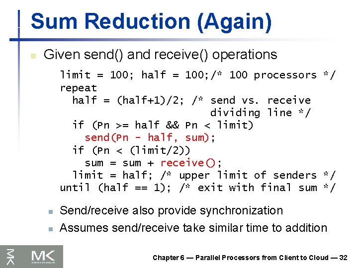
Sum Reduction (Again) n Given send() and receive() operations limit = 100; half = 100; /* 100 processors */ repeat half = (half+1)/2; /* send vs. receive dividing line */ if (Pn >= half && Pn < limit) send(Pn - half, sum); if (Pn < (limit/2)) sum = sum + receive(); limit = half; /* upper limit of senders */ until (half == 1); /* exit with final sum */ n n Send/receive also provide synchronization Assumes send/receive take similar time to addition Chapter 6 — Parallel Processors from Client to Cloud — 32

Grid Computing n Separate computers interconnected by long-haul networks n n n E. g. , Internet connections Work units farmed out, results sent back Can make use of idle time on PCs n E. g. , SETI@home, World Community Grid Chapter 6 — Parallel Processors from Client to Cloud — 33

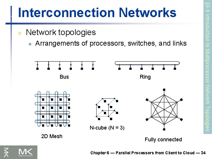
n Network topologies n Arrangements of processors, switches, and links Bus Ring N-cube (N = 3) 2 D Mesh § 6. 8 Introduction to Multiprocessor Network Topologies Interconnection Networks Fully connected Chapter 6 — Parallel Processors from Client to Cloud — 34

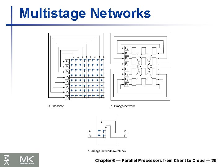
Multistage Networks Chapter 6 — Parallel Processors from Client to Cloud — 35

Network Characteristics n Performance n n Latency per message (unloaded network) Throughput n n n n Link bandwidth Total network bandwidth Bisection bandwidth Congestion delays (depending on traffic) Cost Power Routability in silicon Chapter 6 — Parallel Processors from Client to Cloud — 36

n n Linpack: matrix linear algebra SPECrate: parallel run of SPEC CPU programs n n SPLASH: Stanford Parallel Applications for Shared Memory n n Mix of kernels and applications, strong scaling NAS (NASA Advanced Supercomputing) suite n n Job-level parallelism computational fluid dynamics kernels PARSEC (Princeton Application Repository for Shared Memory Computers) suite n Multithreaded applications using Pthreads and Open. MP § 6. 10 Multiprocessor Benchmarks and Performance Models Parallel Benchmarks Chapter 6 — Parallel Processors from Client to Cloud — 37

Code or Applications? n Traditional benchmarks n n Parallel programming is evolving n n Fixed code and data sets Should algorithms, programming languages, and tools be part of the system? Compare systems, provided they implement a given application E. g. , Linpack, Berkeley Design Patterns Would foster innovation in approaches to parallelism Chapter 6 — Parallel Processors from Client to Cloud — 38

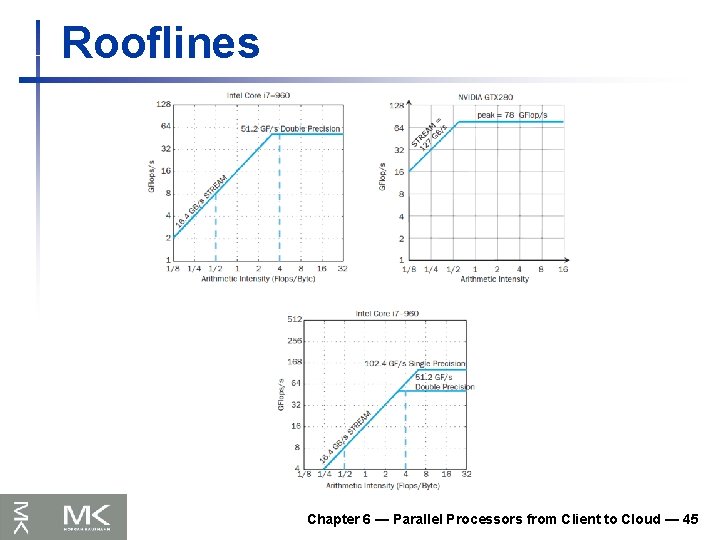
Modeling Performance n Assume performance metric of interest is achievable GFLOPs/sec n n Arithmetic intensity of a kernel n n Measured using computational kernels from Berkeley Design Patterns FLOPs per byte of memory accessed For a given computer, determine n n Peak GFLOPS (from data sheet) Peak memory bytes/sec (using Stream benchmark) Chapter 6 — Parallel Processors from Client to Cloud — 39

Roofline Diagram Attainable GPLOPs/sec = Max ( Peak Memory BW × Arithmetic Intensity, Peak FP Performance ) Chapter 6 — Parallel Processors from Client to Cloud — 40

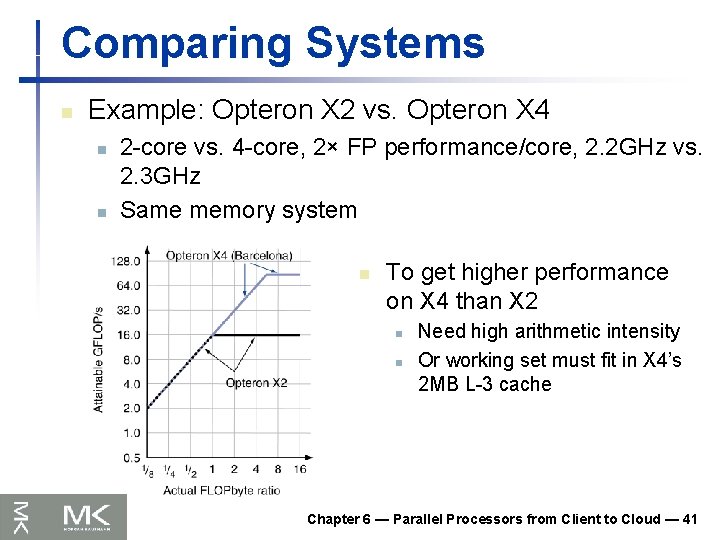
Comparing Systems n Example: Opteron X 2 vs. Opteron X 4 n n 2 -core vs. 4 -core, 2× FP performance/core, 2. 2 GHz vs. 2. 3 GHz Same memory system n To get higher performance on X 4 than X 2 n n Need high arithmetic intensity Or working set must fit in X 4’s 2 MB L-3 cache Chapter 6 — Parallel Processors from Client to Cloud — 41

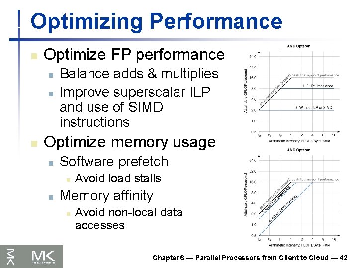
Optimizing Performance n Optimize FP performance n n n Balance adds & multiplies Improve superscalar ILP and use of SIMD instructions Optimize memory usage n Software prefetch n n Avoid load stalls Memory affinity n Avoid non-local data accesses Chapter 6 — Parallel Processors from Client to Cloud — 42

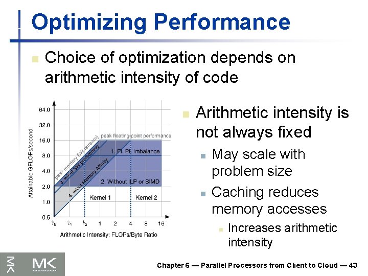
Optimizing Performance n Choice of optimization depends on arithmetic intensity of code n Arithmetic intensity is not always fixed n n May scale with problem size Caching reduces memory accesses n Increases arithmetic intensity Chapter 6 — Parallel Processors from Client to Cloud — 43

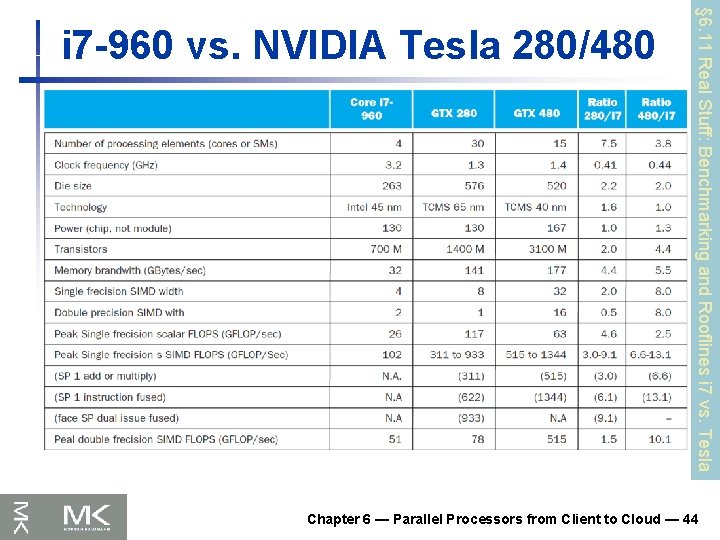
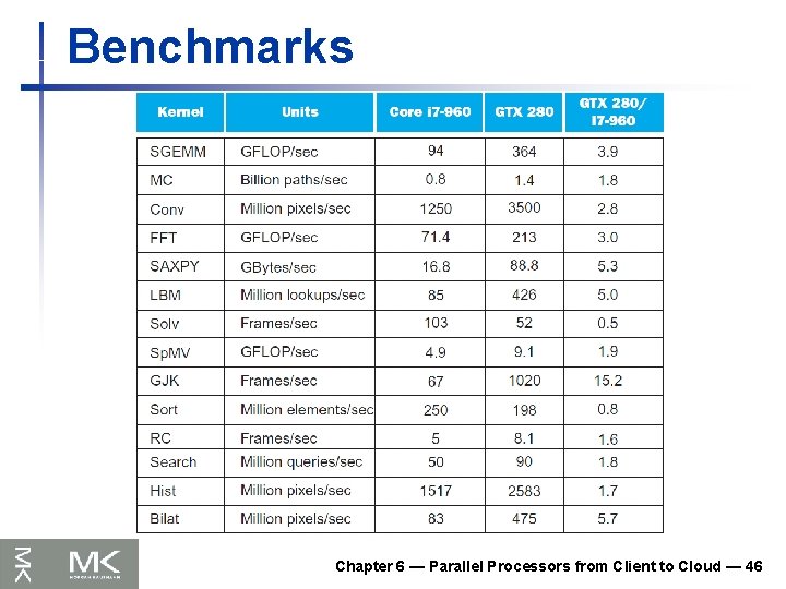
§ 6. 11 Real Stuff: Benchmarking and Rooflines i 7 vs. Tesla i 7 -960 vs. NVIDIA Tesla 280/480 Chapter 6 — Parallel Processors from Client to Cloud — 44

Rooflines Chapter 6 — Parallel Processors from Client to Cloud — 45

Benchmarks Chapter 6 — Parallel Processors from Client to Cloud — 46

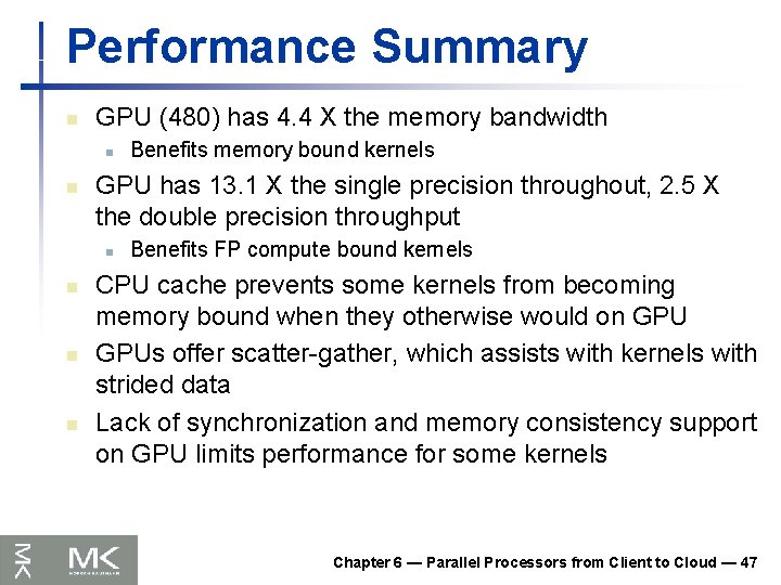
Performance Summary n GPU (480) has 4. 4 X the memory bandwidth n n GPU has 13. 1 X the single precision throughout, 2. 5 X the double precision throughput n n Benefits memory bound kernels Benefits FP compute bound kernels CPU cache prevents some kernels from becoming memory bound when they otherwise would on GPUs offer scatter-gather, which assists with kernels with strided data Lack of synchronization and memory consistency support on GPU limits performance for some kernels Chapter 6 — Parallel Processors from Client to Cloud — 47

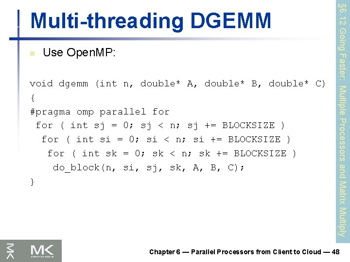
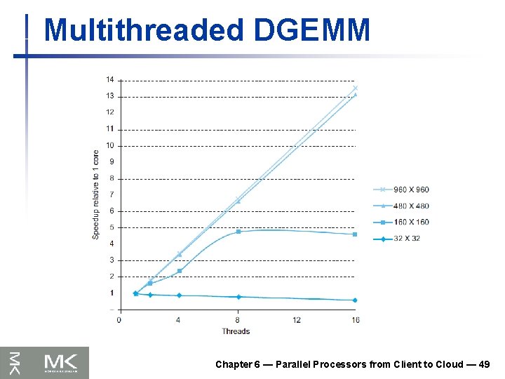
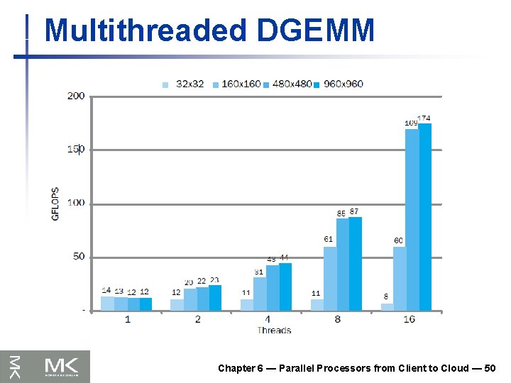
n Use Open. MP: void dgemm (int n, double* A, double* B, double* C) { #pragma omp parallel for ( int sj = 0; sj < n; sj += BLOCKSIZE ) for ( int si = 0; si < n; si += BLOCKSIZE ) for ( int sk = 0; sk < n; sk += BLOCKSIZE ) do_block(n, si, sj, sk, A, B, C); } § 6. 12 Going Faster: Multiple Processors and Matrix Multiply Multi-threading DGEMM Chapter 6 — Parallel Processors from Client to Cloud — 48

Multithreaded DGEMM Chapter 6 — Parallel Processors from Client to Cloud — 49

Multithreaded DGEMM Chapter 6 — Parallel Processors from Client to Cloud — 50

n Amdahl’s Law doesn’t apply to parallel computers n n n Since we can achieve linear speedup But only on applications with weak scaling § 6. 13 Fallacies and Pitfalls Fallacies Peak performance tracks observed performance n n n Marketers like this approach! But compare Xeon with others in example Need to be aware of bottlenecks Chapter 6 — Parallel Processors from Client to Cloud — 51

Pitfalls n Not developing the software to take account of a multiprocessor architecture n Example: using a single lock for a shared composite resource n n Serializes accesses, even if they could be done in parallel Use finer-granularity locking Chapter 6 — Parallel Processors from Client to Cloud — 52

n n Goal: higher performance by using multiple processors Difficulties n n Developing parallel software Devising appropriate architectures § 6. 14 Concluding Remarks Saa. S importance is growing and clusters are a good match Performance per dollar and performance per Joule drive both mobile and WSC Chapter 6 — Parallel Processors from Client to Cloud — 53

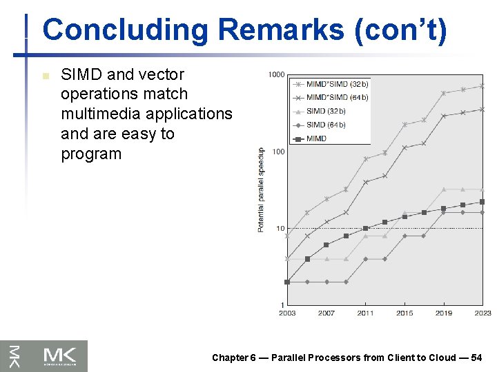
Concluding Remarks (con’t) n SIMD and vector operations match multimedia applications and are easy to program Chapter 6 — Parallel Processors from Client to Cloud — 54