Chapter 6 Overview of Query Processing Author Team1

Chapter 6 Overview of Query Processing Author: “Team-1” Bansariben Thummar, 1809568 Ujjaval Desai, 1856383 Mahavir Chhasatiya, 1800725 Instructor: Dr. Andrew Yang Department: Computer Science Course: CSCI 5533 Distributed Information Systems

Outline Query Processing Problem Objective of Query Processing Complexity of Relational Algebra Operations Characterization of Query Processors Layers of Query Processing Conclusion 1

Overview of Query Processing What is Query ? A query is a statement requesting the retrieval of information. The portion of a DML (Data Manipulation Language) that involves information retrieval is called a query language. 2

Overview of Query Processing Alternative ways of evaluating a given query Equivalent expressions Different algorithms for each operation An evaluation plan defines exactly what algorithm is used for each operation, and how the execution of the operations is coordinated. 3

Overview of Query Processing What is Query Processor? In relational database technology, users perform the task of data processing and data manipulation with the help of high level nonprocedural language (e. g. SQL). This high-level query hides the low-level details from the user about the physical organization of the data and presents such an environment so that the user can handle the tasks of even complex queries in an easy, concise and simple fashion. The inner procedure of query-task is performed by a DBMS module called a Query Processor. Hence the users are relieved from query optimization which is a time consuming task that is actually performed by the query processor. 4

Overview of Query Processing What is Query Processor? Understanding Query processing in distributed database environments is very difficult instead of centralized database, because there are many elements or parameters involved that affect the overall performance of distributed queries. Moreover, in distributed environment, the query processor may have to access in many sites. Thus, query response time may become very high. That is why, Query processing problem is divided into several subproblems/ steps which are easier to solve individually. 5

Overview of Query Processing Problem Main Function/Objective of a Query Processor • Main function of a query processor is to transform a highlevel-query (also called calculus query) into an equivalent lower-level query (also called algebraic query). • The conversion must be correct and efficient. The conversion will be correct if low-level query has the same semantics as the original query, i. e. if both queries produce the same result. 6

Overview of Query Processing Main Problems of Query Processing Main problem of query processing is query optimization. It is a time consuming task, because many execution strategies are involved to minimize (optimize) computer recourse consumption. Total cost also affects query processing. Cost depends on the time required for processing operations of the query at various sites, utilization of various computer resources etc, time needed for exchanging data between sites participating in the execution of the query etc. Time and space required to process the query is also an important factor for the performance of the query processing. 7

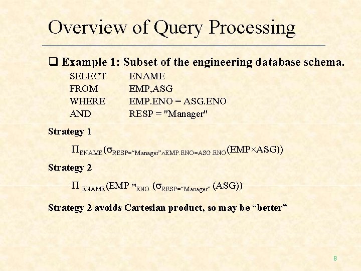
Overview of Query Processing Example 1: Subset of the engineering database schema. SELECT FROM WHERE AND ENAME EMP, ASG EMP. ENO = ASG. ENO RESP = "Manager" Strategy 1 ENAME( RESP=“Manager” EMP. ENO=ASG. ENO(EMP×ASG)) Strategy 2 ENAME(EMP ⋈ENO ( RESP=“Manager” (ASG)) Strategy 2 avoids Cartesian product, so may be “better” 8

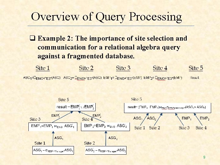
Overview of Query Processing Example 2: The importance of site selection and communication for a relational algebra query against a fragmented database. 9

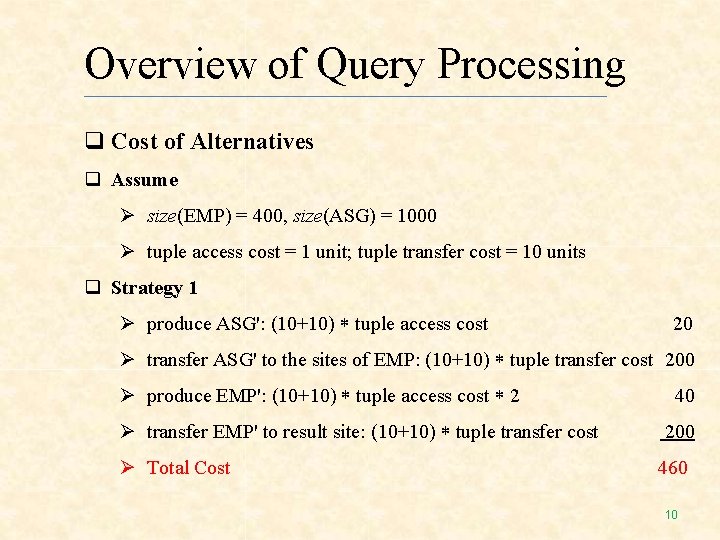
Overview of Query Processing Cost of Alternatives Assume size(EMP) = 400, size(ASG) = 1000 tuple access cost = 1 unit; tuple transfer cost = 10 units Strategy 1 produce ASG': (10+10) tuple access cost 20 transfer ASG' to the sites of EMP: (10+10) tuple transfer cost 200 produce EMP': (10+10) tuple access cost 2 transfer EMP' to result site: (10+10) tuple transfer cost Total Cost 40 200 460 10

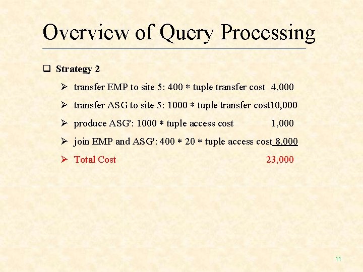
Overview of Query Processing Strategy 2 transfer EMP to site 5: 400 tuple transfer cost 4, 000 transfer ASG to site 5: 1000 tuple transfer cost 10, 000 produce ASG': 1000 tuple access cost 1, 000 join EMP and ASG': 400 20 tuple access cost 8, 000 Total Cost 23, 000 11

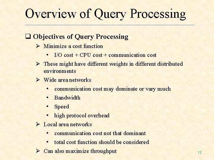
Overview of Query Processing Objectives of Query Processing Minimize a cost function • I/O cost + CPU cost + communication cost These might have different weights in different distributed environments Wide area networks • communication cost may dominate or vary much • Bandwidth • Speed • high protocol overhead Local area networks • communication cost not that dominant • total cost function should be considered Can also maximize throughput 12

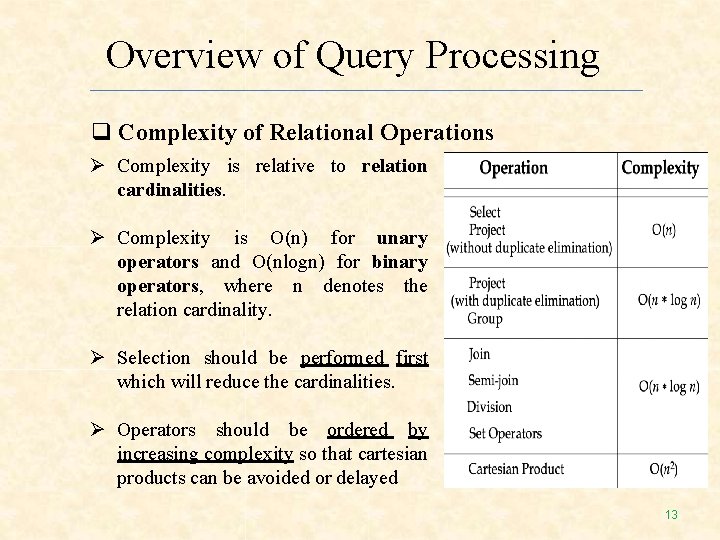
Overview of Query Processing Complexity of Relational Operations Complexity is relative to relation cardinalities. Complexity is O(n) for unary operators and O(nlogn) for binary operators, where n denotes the relation cardinality. Selection should be performed first which will reduce the cardinalities. Operators should be ordered by increasing complexity so that cartesian products can be avoided or delayed 13

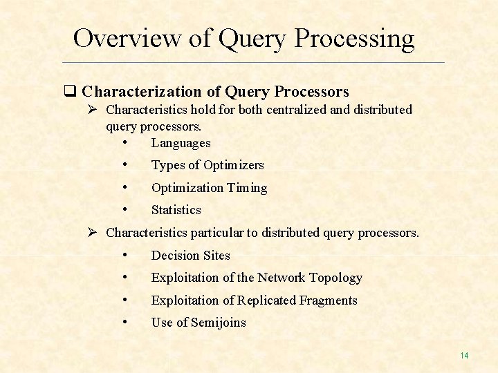
Overview of Query Processing Characterization of Query Processors Characteristics hold for both centralized and distributed query processors. • Languages • Types of Optimizers • Optimization Timing • Statistics Characteristics particular to distributed query processors. • Decision Sites • Exploitation of the Network Topology • Exploitation of Replicated Fragments • Use of Semijoins 14

Overview of Query Processing Characteristics of Query Processor: Languages Input language to the query processor is based on high-level relational DBMS, i. e. input is in Relational Calculus query. On the other hand, output language is based on lower-level relational DMBS, i. e. output is in Relational Algebraic query. The operations of the output language are implemented directly in the computer system. Query processing must perform efficient mapping from the input language to the output language. 15

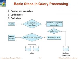
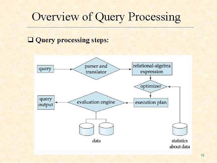
Overview of Query Processing Query processing steps: 16

Overview of Query Processing Characteristics of Query Processor: Types Of Optimizers Goal of Optimizer: It aims to choose the “best” point in the solution space of all possible execution strategies in terms of time and space complexity. Problem to tackle: • Solution space can be large. • Similar strategies due to small number of relations. • The problem becomes worse as the number of relations or fragments increases. Role of Optimizer: • To search the solution space. • Exhaustively predict the cost of each strategy. • Select the strategy with minimum cost. Two types of optimization: • Cost based optimization • Heuristics optimization (Logical) 17

Overview of Query Processing Characteristics of Query Processor: Types Of Optimizers (cont. ) Cost based optimization • Based on the cost of the query. • This method mainly uses the statistics like record size, number of records per block, number of blocks, table size etc. • Advantage: Consistently chooses the best solution • Disadvantage: Exponential time and space complexity owing to the large solution space. • Algorithm paradigms used in cost based optimization. o Dynamic Programming, Left Deep Trees etc. 18

Overview of Query Processing Characteristics of Query Processor: Types Of Optimizers (cont. ) Heuristic Optimization (Logical) • This method is also known as rule based optimization. • This is based on the equivalence rule on relational expressions; hence the number of combination of queries get reduces here. Hence the cost of the query too reduces. • Advantage: Polynomial time and space complexity better than Cost based optimization. • Disadvantage: These algorithms do not necessarily produce the best query plan. 19

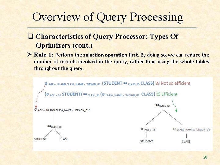
Overview of Query Processing Characteristics of Query Processor: Types Of Optimizers (cont. ) Rule-1: Perform the selection operation first. By doing so, we can reduce the number of records involved in the query, rather than using the whole tables throughout the query. 20

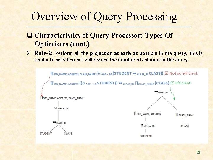
Overview of Query Processing Characteristics of Query Processor: Types Of Optimizers (cont. ) Rule-2: Perform all the projection as early as possible in the query. This is similar to selection but will reduce the number of columns in the query. 21

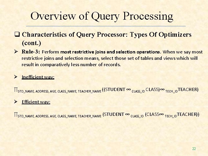
Overview of Query Processing Characteristics of Query Processor: Types Of Optimizers (cont. ) Rule-3: Perform most restrictive joins and selection operations. When we say most restrictive joins and selection means, select those set of tables and views which will result in comparatively less number of records. Inefficient way: ∏STD_NAME, ADDRESS, AGE, CLASS_NAME, TEACHER_NAME ((STUDENT ∞ CLASS_ID CLASS)∞ TECH_IDTEACHER) Efficient way: ∏STD_NAME, ADDRESS, AGE, CLASS_NAME, TEACHER_NAME (STUDENT ∞ CLASS_ID (CLASS∞ TECH_IDTEACHER)) 22

Overview of Query Processing Characteristics of Query Processor: Optimization Timing The actual time required to optimize the execution of a query is an important factor. If less time is required, then it is the best solution for query processing. Optimized at different times relative to the actual time of query execution. Static • Optimization can be done before executing the query. • Determines the estimated size of the intermediate relations of a strategy. • Sizes of the intermediate relations of a strategy are estimated using database statistics. • Not always accurate, there might be estimation errors. • Appropriate for the exhaustive search method. 23

Overview of Query Processing Characteristics of Query Processor: Optimization Timing (cont. ) Dynamic • Optimization can be done at query execution time. • Determines the actual size of the intermediate relations of a strategy. • Sizes of the intermediate relations of a strategy are NOT estimated using database statistics. • Main advantage over static optimization is actual sizes of intermediate relations are available to the query processor • Appropriate for the ad-hoc queries. Hybrid • Uses both static and dynamic optimization. • By default static optimization is used. • If the error in Estimated size > Actual size, reoptimize dynamically. 24

Overview of Query Processing Characteristics of Query Processor: Statistics The effectiveness of query optimization relies on statistical information of the database, i. e. how many fragments query will be needed, which operation should be done first, size and number of distinct values of each attribute of the relation, histograms of the attributes for minimizing probability error etc. Table statistics Number of rows, Number of blocks, Average row length. Column statistics Number of distinct values (NDV) in column, Number of nulls in column, Data distribution (histogram). System statistics I/O performance and utilization, CPU performance and utilization. Common assumptions • Independence between different attribute values • Uniform distribution of attribute values within their domain 25

Overview of Query Processing Characteristics of Query Processor: Decision Sites In a distributed database, several sites may participate for answering the query. Most systems use centralized decision approach, in which a single site generates the strategy. However, the decision process could be distributed among various sites. Centralized • Single site determines the “best” schedule • Simple • Need knowledge about the entire distributed database Distributed • Cooperation among sites to determine the schedule • Need only local information • Cost of cooperation Hybrid • One site determines the global schedule • Each site optimizes the local subqueries 26

Overview of Query Processing Characteristics of Query Processor: Exploitation of Network Topology Distributed query processor uses computer network, so its performance depends also on which topology it is using. The cost function, speed, utilization of various network resources are important factors for executing query processor in a distributed environment. Wide area networks (WAN) – point-to-point • Characteristics Low bandwidth Low speed High protocol overhead • Communication cost will dominate; ignore all other cost factors • Global schedule to minimize communication cost • Local schedules according to centralized query 27 optimization

Overview of Query Processing Characteristics of Query Processor: Exploitation of Network Topology (cont. ) Local area networks (LAN) • Communication cost is not dominant. • Total cost function should be considered. • Broadcasting can be exploited (joins). • Special algorithms exist for star networks. 28

Overview of Query Processing Characteristics of Query Processor: Exploitation of Replicated Fragments A distributed relation is usually divided into relation fragments. Distributed queries expressed on global relations are mapped into queries on physical fragments of relations by translating relations into fragments. We call this process localization because its main function is to localize the data involved in the query. For higher reliability and better read performance, it is useful to have fragments replicated at different sites. 29

Overview of Query Processing Characteristics of Query Processor: Use of Semi-join operation In distributed system, it is better to use semi-join operation instead of join operation for minimizing data communication. Advantage: • Reduces the size of the operand relation. Disadvantage: • Increase in number of messages and local processing time. Use : • Wide area networks makes extensive use of semijoins. • R* which assume faster networks does not employ semijoins as joins has lower local processing cost. 30

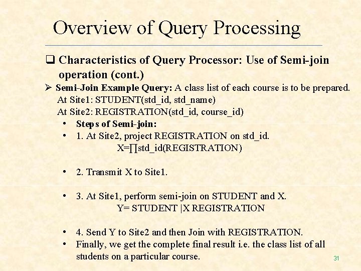
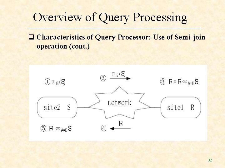
Overview of Query Processing Characteristics of Query Processor: Use of Semi-join operation (cont. ) Semi-Join Example Query: A class list of each course is to be prepared. At Site 1: STUDENT(std_id, std_name) At Site 2: REGISTRATION(std_id, course_id) • Steps of Semi-join: • 1. At Site 2, project REGISTRATION on std_id. X=∏std_id(REGISTRATION) • 2. Transmit X to Site 1. • 3. At Site 1, perform semi-join on STUDENT and X. Y= STUDENT |X REGISTRATION • 4. Send Y to Site 2 and then Join with REGISTRATION. • Finally, we get the complete final result i. e. the class list of all students on a particular course. 31

Overview of Query Processing Characteristics of Query Processor: Use of Semi-join operation (cont. ) 32

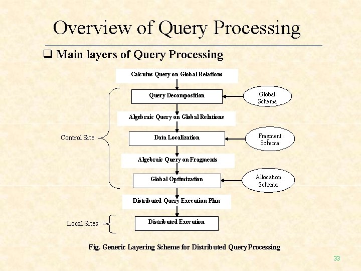
Overview of Query Processing Main layers of Query Processing Calculus Query on Global Relations Query Decomposition Global Schema Algebraic Query on Global Relations Control Site Data Localization Fragment Schema Algebraic Query on Fragments Global Optimization Allocation Schema Distributed Query Execution Plan Local Sites Distributed Execution Fig. Generic Layering Scheme for Distributed Query Processing 33

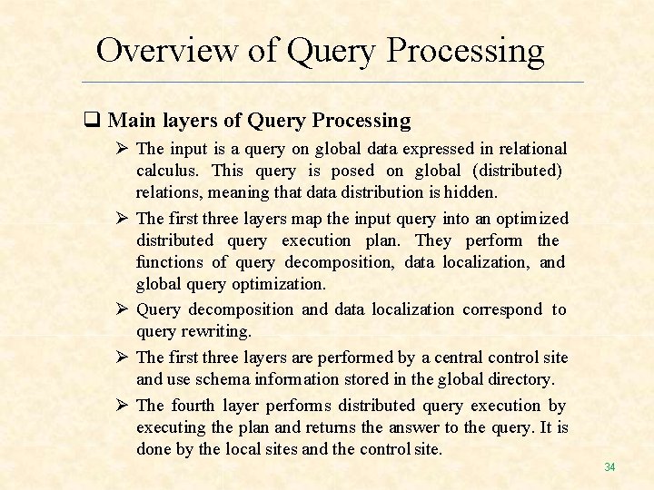
Overview of Query Processing Main layers of Query Processing The input is a query on global data expressed in relational calculus. This query is posed on global (distributed) relations, meaning that data distribution is hidden. The first three layers map the input query into an optimized distributed query execution plan. They perform the functions of query decomposition, data localization, and global query optimization. Query decomposition and data localization correspond to query rewriting. The first three layers are performed by a central control site and use schema information stored in the global directory. The fourth layer performs distributed query execution by executing the plan and returns the answer to the query. It is done by the local sites and the control site. 34

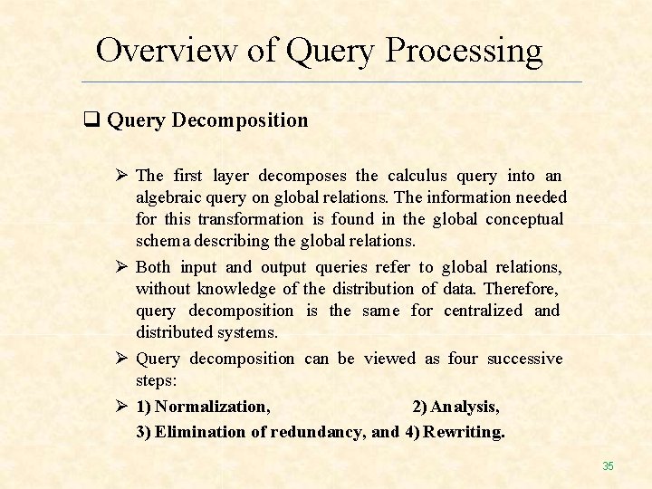
Overview of Query Processing Query Decomposition The first layer decomposes the calculus query into an algebraic query on global relations. The information needed for this transformation is found in the global conceptual schema describing the global relations. Both input and output queries refer to global relations, without knowledge of the distribution of data. Therefore, query decomposition is the same for centralized and distributed systems. Query decomposition can be viewed as four successive steps: 1) Normalization, 2) Analysis, 3) Elimination of redundancy, and 4) Rewriting. 35

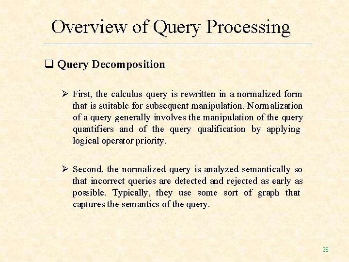
Overview of Query Processing Query Decomposition First, the calculus query is rewritten in a normalized form that is suitable for subsequent manipulation. Normalization of a query generally involves the manipulation of the query quantifiers and of the query qualification by applying logical operator priority. Second, the normalized query is analyzed semantically so that incorrect queries are detected and rejected as early as possible. Typically, they use some sort of graph that captures the semantics of the query. 36

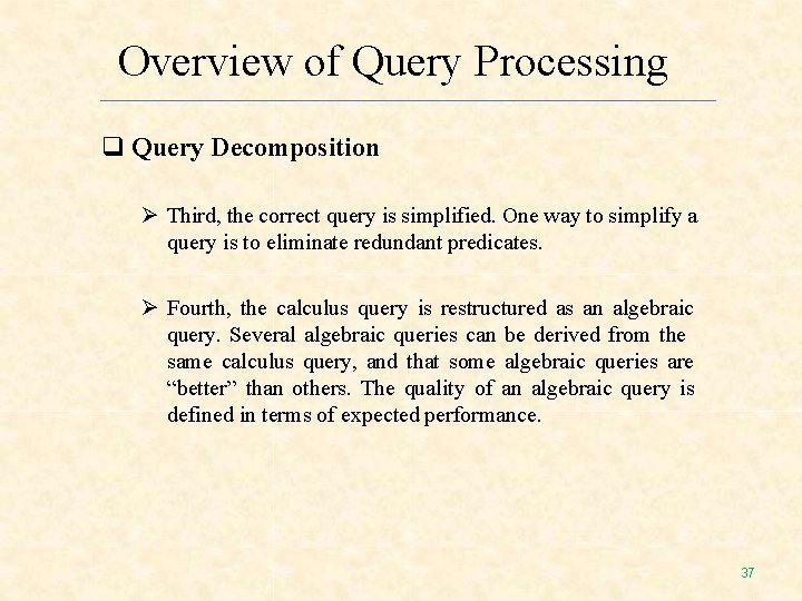
Overview of Query Processing Query Decomposition Third, the correct query is simplified. One way to simplify a query is to eliminate redundant predicates. Fourth, the calculus query is restructured as an algebraic query. Several algebraic queries can be derived from the same calculus query, and that some algebraic queries are “better” than others. The quality of an algebraic query is defined in terms of expected performance. 37

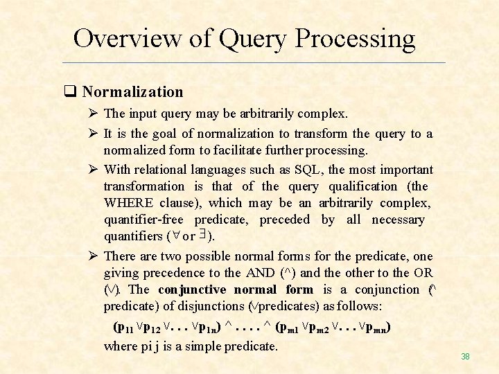
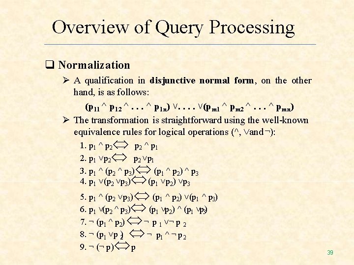
Overview of Query Processing Normalization The input query may be arbitrarily complex. It is the goal of normalization to transform the query to a normalized form to facilitate further processing. With relational languages such as SQL, the most important transformation is that of the query qualification (the WHERE clause), which may be an arbitrarily complex, quantifier-free predicate, preceded by all necessary quantifiers ( or ). There are two possible normal forms for the predicate, one giving precedence to the AND (^) and the other to the OR (˅). The conjunctive normal form is a conjunction (^ predicate) of disjunctions (˅predicates) as follows: (p 11 ˅p 12 ˅. . . ˅p 1 n) ^. . ^ (pm 1 ˅pm 2 ˅. . . ˅pmn) where pi j is a simple predicate. 38

Overview of Query Processing Normalization A qualification in disjunctive normal form, on the other hand, is as follows: (p 11 ^ p 12 ^. . . ^ p 1 n) ˅. . ˅(pm 1 ^ pm 2 ^. . . ^ pmn) The transformation is straightforward using the well-known equivalence rules for logical operations (^, ˅and ¬): 1. p 1 ^ p 2 ^ p 1 2. p 1 ˅p 2 ˅p 1 3. p 1 ^ (p 2 ^ p 3) (p 1 ^ p 2) ^ p 3 4. p 1 ˅(p 2 ˅p 3) (p 1 ˅p 2) ˅p 3 5. p ^ (p ˅p ) (p ^ p ) ˅(p ^ p ) 6. p ˅(p ^ p ) (p ˅p ) ^ (p ˅p ) 7. ¬ (p ^ p ) ¬ p ˅¬ p 8. ¬ (p ˅p ) ¬ p ^ ¬ p 9. ¬ (¬ p) p 1 2 1 3 2 3 1 1 2 1 2 1 2 3 3 39

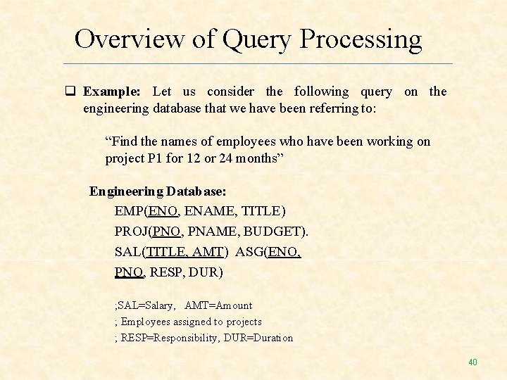
Overview of Query Processing Example: Let us consider the following query on the engineering database that we have been referring to: “Find the names of employees who have been working on project P 1 for 12 or 24 months” Engineering Database: EMP(ENO, ENAME, TITLE) PROJ(PNO, PNAME, BUDGET). SAL(TITLE, AMT) ASG(ENO, PNO, RESP, DUR) ; SAL=Salary, AMT=Amount ; Employees assigned to projects ; RESP=Responsibility, DUR=Duration 40

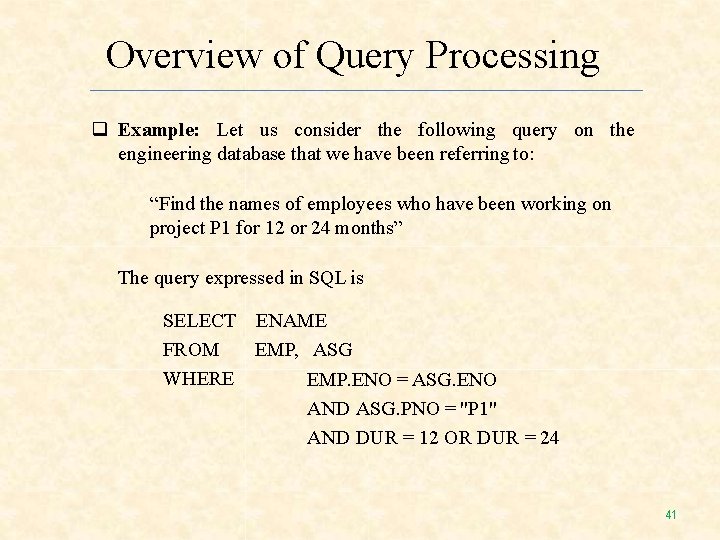
Overview of Query Processing Example: Let us consider the following query on the engineering database that we have been referring to: “Find the names of employees who have been working on project P 1 for 12 or 24 months” The query expressed in SQL is SELECT ENAME FROM EMP, ASG WHERE EMP. ENO = ASG. ENO AND ASG. PNO = "P 1" AND DUR = 12 OR DUR = 24 41

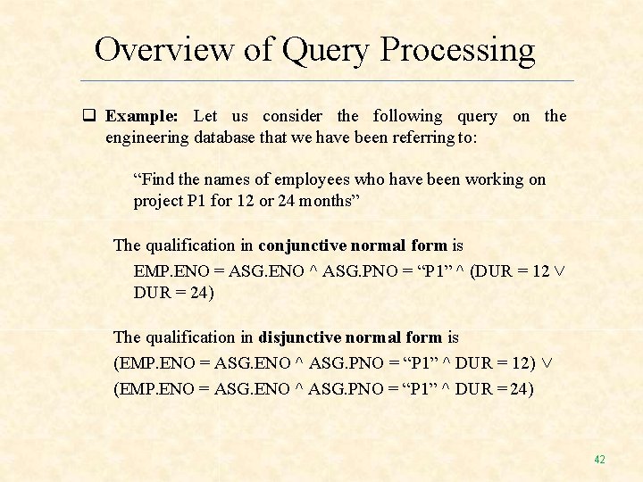
Overview of Query Processing Example: Let us consider the following query on the engineering database that we have been referring to: “Find the names of employees who have been working on project P 1 for 12 or 24 months” The qualification in conjunctive normal form is EMP. ENO = ASG. ENO ^ ASG. PNO = “P 1” ^ (DUR = 12 ˅ DUR = 24) The qualification in disjunctive normal form is (EMP. ENO = ASG. ENO ^ ASG. PNO = “P 1” ^ DUR = 12) ˅ (EMP. ENO = ASG. ENO ^ ASG. PNO = “P 1” ^ DUR = 24) 42

Overview of Query Processing Analysis Query analysis enables rejection of normalized queries for which further processing is either impossible or unnecessary. The main reasons for rejection are that the query is type incorrect or semantically incorrect. A query is type incorrect if any of its attribute or relation names are not defined in the global schema, or if operations are being applied to attributes of the wrong type. The technique used to detect type incorrect queries is similar to type checking for programming languages. 43

Overview of Query Processing Analysis Example: The following SQL query on the engineering database is type incorrect for two reasons. First, attribute E# is not declared in the schema. Second, the operation “>200” is incompatible with the type string of ENAME. SELECT E# FROM EMP WHERE ENAME > 200 44

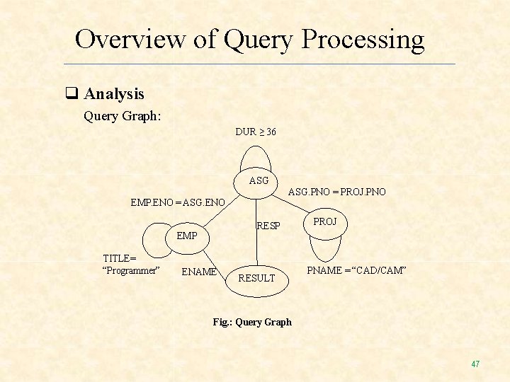
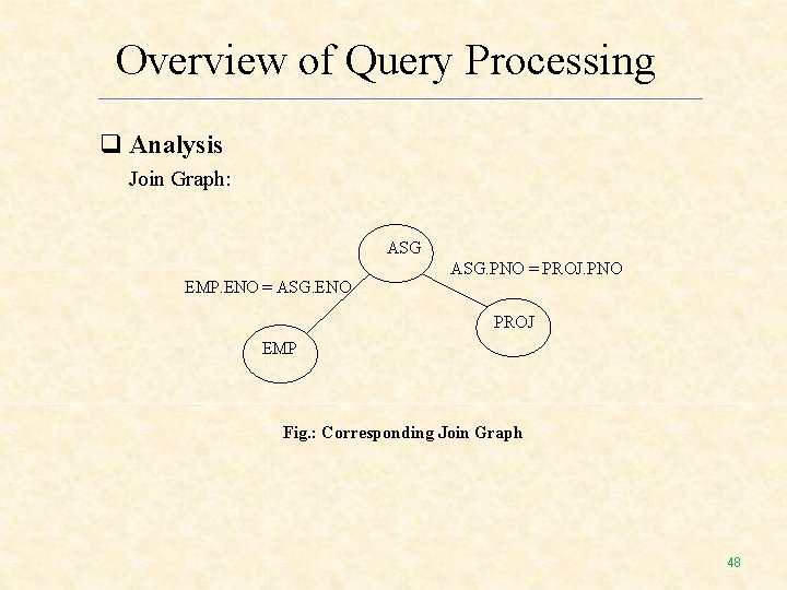
Overview of Query Processing Analysis A query is semantically incorrect if its components do not contribute in any way to the generation of the result. This is based on the representation of the query as a graph, called a query graph or connection graph. In a query graph, one node indicates the result relation, and any other node indicates an operand relation. An edge between two nodes one of which does not correspond to the result represents a join, whereas an edge whose destination node is the result represents a project. An important subgraph of the query graph is the join graph, in which only the joins are considered. 45

Overview of Query Processing Analysis Example: Let us consider the following query: “Find the names and responsibilities of programmers who have been working on the CAD/CAM project for more than 3 years. ” The query expressed in SQL is SELECT ENAME, RESP FROM EMP, ASG, PROJ WHERE EMP. ENO = ASG. ENO AND ASG. PNO = PROJ. PNO AND PNAME = "CAD/CAM" AND DUR ≥ 36 AND TITLE = "Programmer“ 46

Overview of Query Processing Analysis Query Graph: DUR ≥ 36 ASG. PNO = PROJ. PNO EMP. ENO = ASG. ENO RESP EMP TITLE= “Programmer” ENAME RESULT PROJ PNAME = “CAD/CAM” Fig. : Query Graph 47

Overview of Query Processing Analysis Join Graph: ASG EMP. ENO = ASG. ENO ASG. PNO = PROJ. PNO PROJ EMP Fig. : Corresponding Join Graph 48

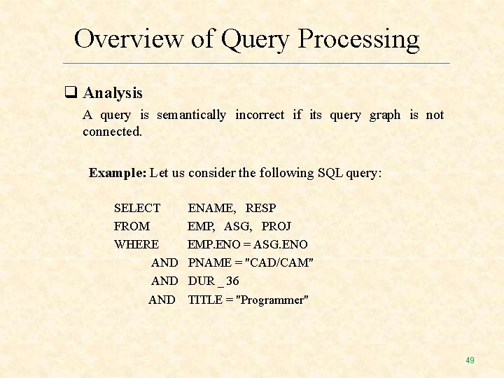
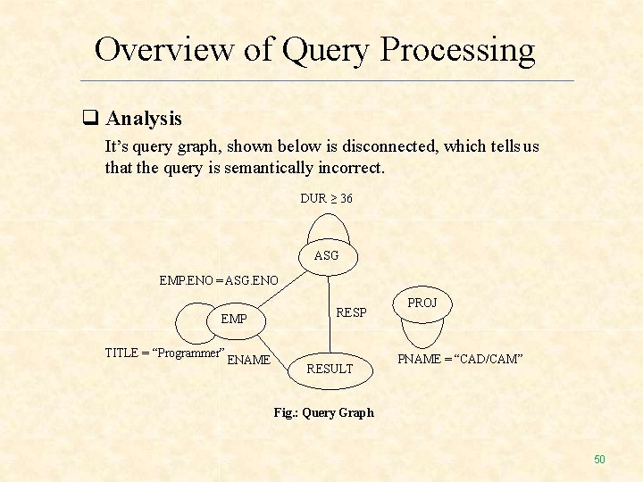
Overview of Query Processing Analysis A query is semantically incorrect if its query graph is not connected. Example: Let us consider the following SQL query: SELECT FROM WHERE AND AND ENAME, RESP EMP, ASG, PROJ EMP. ENO = ASG. ENO PNAME = "CAD/CAM" DUR _ 36 TITLE = "Programmer" 49

Overview of Query Processing Analysis It’s query graph, shown below is disconnected, which tells us that the query is semantically incorrect. DUR ≥ 36 ASG EMP. ENO = ASG. ENO EMP TITLE = “Programmer” ENAME RESP RESULT PROJ PNAME = “CAD/CAM” Fig. : Query Graph 50

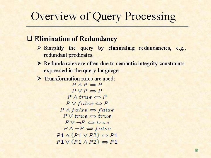
Overview of Query Processing Elimination of Redundancy Simplify the query by eliminating redundancies, e. g. , redundant predicates. Redundancies are often due to semantic integrity constraints expressed in the query language. Transformation rules are used: 51

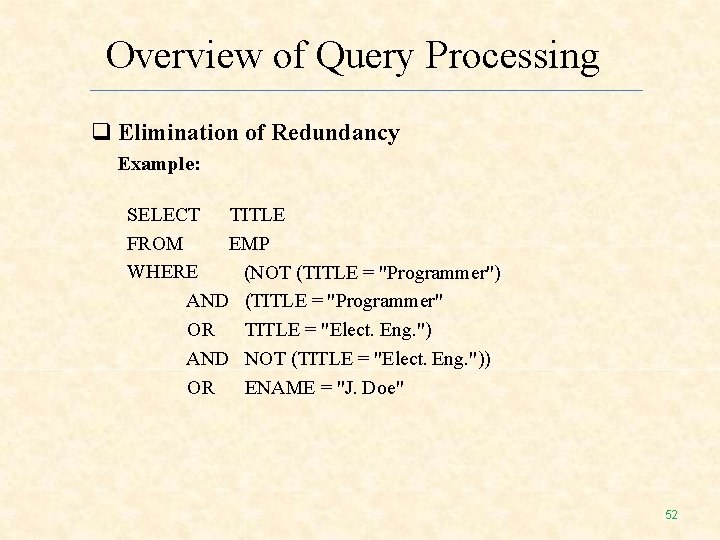
Overview of Query Processing Elimination of Redundancy Example: SELECT TITLE FROM EMP WHERE (NOT (TITLE = "Programmer") AND (TITLE = "Programmer" OR TITLE = "Elect. Eng. ") AND NOT (TITLE = "Elect. Eng. ")) OR ENAME = "J. Doe" 52

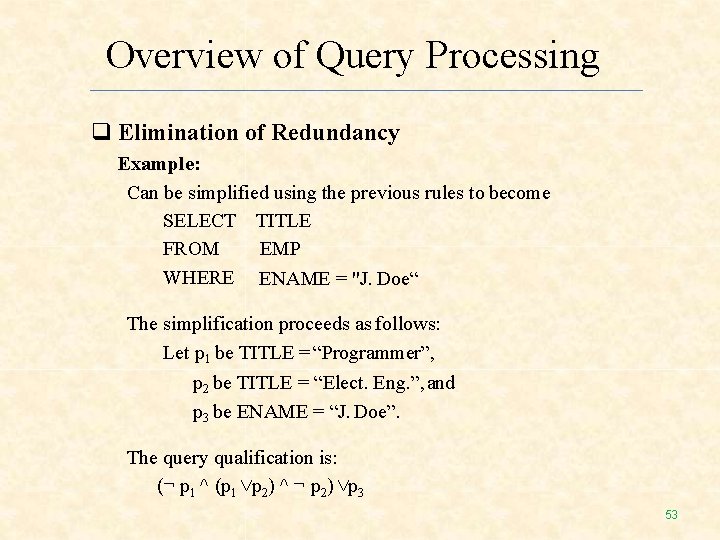
Overview of Query Processing Elimination of Redundancy Example: Can be simplified using the previous rules to become SELECT TITLE FROM EMP WHERE ENAME = "J. Doe“ The simplification proceeds as follows: Let p 1 be TITLE = “Programmer”, p 2 be TITLE = “Elect. Eng. ”, and p 3 be ENAME = “J. Doe”. The query qualification is: (¬ p 1 ^ (p 1 ˅p 2) ^ ¬ p 2) ˅p 3 53

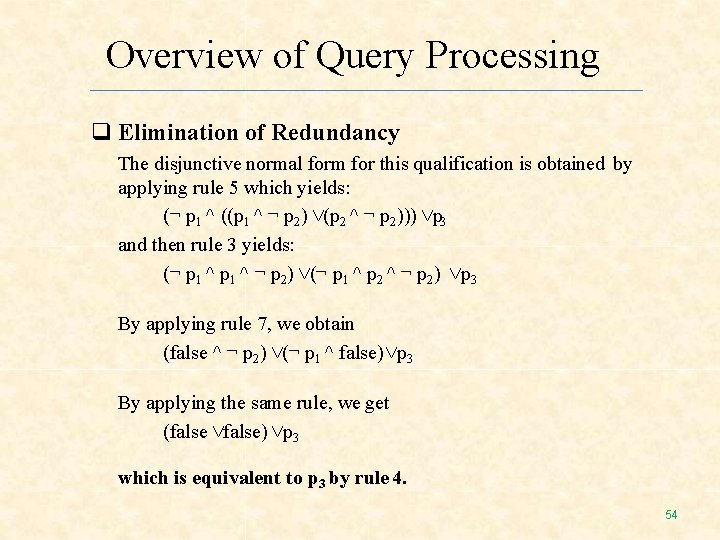
Overview of Query Processing Elimination of Redundancy The disjunctive normal form for this qualification is obtained by applying rule 5 which yields: (¬ p 1 ^ ((p 1 ^ ¬ p 2) ˅(p 2 ^ ¬ p 2))) ˅p 3 and then rule 3 yields: (¬ p 1 ^ ¬ p 2) ˅(¬ p 1 ^ p 2 ^ ¬ p 2) ˅p 3 By applying rule 7, we obtain (false ^ ¬ p 2) ˅(¬ p 1 ^ false) ˅p 3 By applying the same rule, we get (false ˅false) ˅p 3 which is equivalent to p 3 by rule 4. 54

Overview of Query Processing Rewriting The last step of query decomposition rewrites the query in relational algebra. For the sake of clarity it is customary to represent the relational algebra query graphically by an operator tree. An operator tree is a tree in which a leaf node is a relation stored in the database, and a non-leaf node is an intermediate relation produced by a relational algebra operator. The sequence of operations is directed from the leaves to the root, which represents the answer to the query. 55

Overview of Query Processing Rewriting The transformation of a tuple relational calculus query into an operator tree can easily be achieved as follows: First, a different leaf is created for each different tuple variable (corresponding to a relation). In SQL, the leaves are immediately available in the FROM clause. Second, the root node is created as a project operation involving the result attributes. These are found in the SELECT clause in SQL. Third, the qualification (SQL WHERE clause) is translated into the appropriate sequence of relational operations (select, join, union, etc. ) going from the leaves to the root. The sequence can be given directly by the order of appearance of the predicates and operators. 56

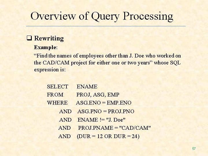
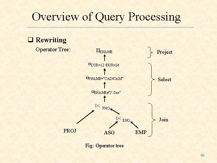
Overview of Query Processing Rewriting Example: “Find the names of employees other than J. Doe who worked on the CAD/CAM project for either one or two years” whose SQL expression is: SELECT FROM WHERE AND AND ENAME PROJ, ASG, EMP ASG. ENO = EMP. ENO ASG. PNO = PROJ. PNO ENAME != "J. Doe" PROJ. PNAME = "CAD/CAM" (DUR = 12 OR DUR = 24) 57

Overview of Query Processing Rewriting Operator Tree: ΠENAME Project σDUR=12 ˅DUR=24 σPNAME=”CAD/CAM” Select σENAME≠”J. Doe” PNO Join ENO PROJ ASG EMP Fig: Operator tree 58

Overview of Query Processing Localization of Distributed Data Output of the first layer is an algebraic query on distributed relations which is input to the second layer. The main role of this layer is to localize the query’s data using data distribution information. We know that relations are fragmented and stored in disjoint subsets, called fragments where each fragment is stored at different site. 59

Overview of Query Processing Localization of Distributed Data This layer determines which fragments are involved in the query and transforms the distributed query into a fragment query. A naive way to localize a distributed query is to generate a query where each global relation is substituted by its localization program. This can be viewed as replacing the leaves of the operator tree of the distributed query with subtrees corresponding to the localization programs. We call the query obtained this way the localized query. 60

Overview of Query Processing Global Query Optimization The input to the third layer is a fragment algebraic query. The goal of this layer is to find an execution strategy for the algebraic fragment query which is close to optimal. Query optimization consists of i)Finding the best ordering of operations in the fragment query, ii) Finding the communication operations which minimize a cost function. 61

Overview of Query Processing Global Query Optimization The cost function refers to computing resources such as disk space, disk I/Os, buffer space, CPU cost, communication cost, and so on. Query optimization is achieved through the semi-join operator instead of join operators. 62

Overview of Query Processing Distributed Execution The last layer is performed by all the sites having fragments involved in the query. Each subquery, called a local query, is executing at one site. It is then optimized using the local schema of the site. 63

Thank you 64

Class Exercise Questions 1) Which of the characteristic is not hold by both centralized and distributed query processors? A) Database Statistics B) Types of Optimizers C) Decision Sites D) Optimization Timing 2) Which operation is performed for reducing cardinalities to the least extent? A) Projection B) Selection C) Group D) Semi-Join 3) Which of the following is not the function of optimizer? A) Searching in the solution space. B) Predicting the cost of each strategy. C) Mapping the results with each strategy. D) Selecting the strategy with minimum cost. 65

Class Exercise Questions 4) Which of the following is one of the rule of Heuristic Optimization? A) Perform the selection operation first and projection operation last. B) Perform the selection operation last and projection operation first. C) Perform projection operation as early as possible. D) None 5) Which of the following is the common assumption in database statistics? A) No dependency between different attribute values. B) Dependency between different attribute values. C) Distinct values of each attribute of the relation. D) Histograms of the attributes for minimizing probability error. 66