Lecture 2 Single Processor Machines Memory Hierarchies and

Lecture 2 Single Processor Machines: Memory Hierarchies and Processor Features UCSB CS 240 A, Winter 2013 Modified from Demmel/Yelick’s slides 1

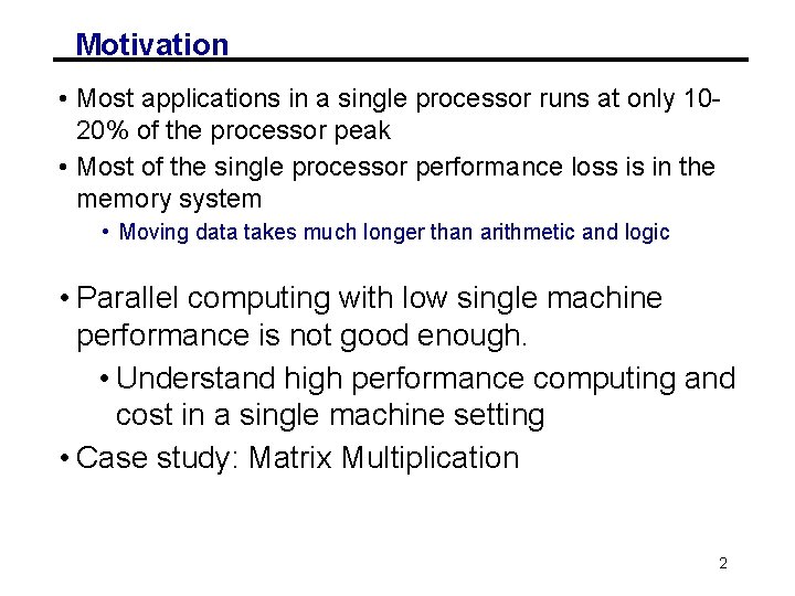
Motivation • Most applications in a single processor runs at only 1020% of the processor peak • Most of the single processor performance loss is in the memory system • Moving data takes much longer than arithmetic and logic • Parallel computing with low single machine performance is not good enough. • Understand high performance computing and cost in a single machine setting • Case study: Matrix Multiplication 2

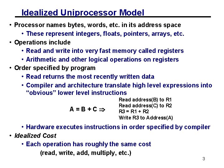
Idealized Uniprocessor Model • Processor names bytes, words, etc. in its address space • These represent integers, floats, pointers, arrays, etc. • Operations include • Read and write into very fast memory called registers • Arithmetic and other logical operations on registers • Order specified by program • Read returns the most recently written data • Compiler and architecture translate high level expressions into “obvious” lower level instructions A=B+C Read address(B) to R 1 Read address(C) to R 2 R 3 = R 1 + R 2 Write R 3 to Address(A) • Hardware executes instructions in order specified by compiler • Idealized Cost • Each operation has roughly the same cost (read, write, add, multiply, etc. ) 3

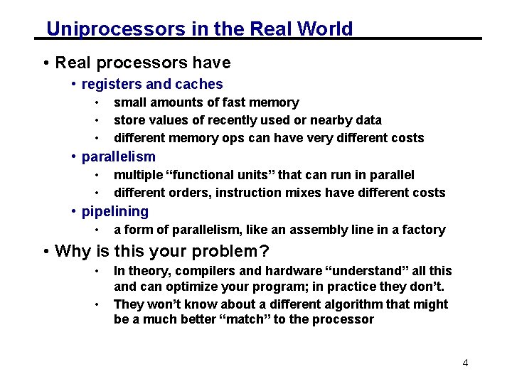
Uniprocessors in the Real World • Real processors have • registers and caches • • • small amounts of fast memory store values of recently used or nearby data different memory ops can have very different costs • parallelism • • multiple “functional units” that can run in parallel different orders, instruction mixes have different costs • pipelining • a form of parallelism, like an assembly line in a factory • Why is this your problem? • • In theory, compilers and hardware “understand” all this and can optimize your program; in practice they don’t. They won’t know about a different algorithm that might be a much better “match” to the processor 4

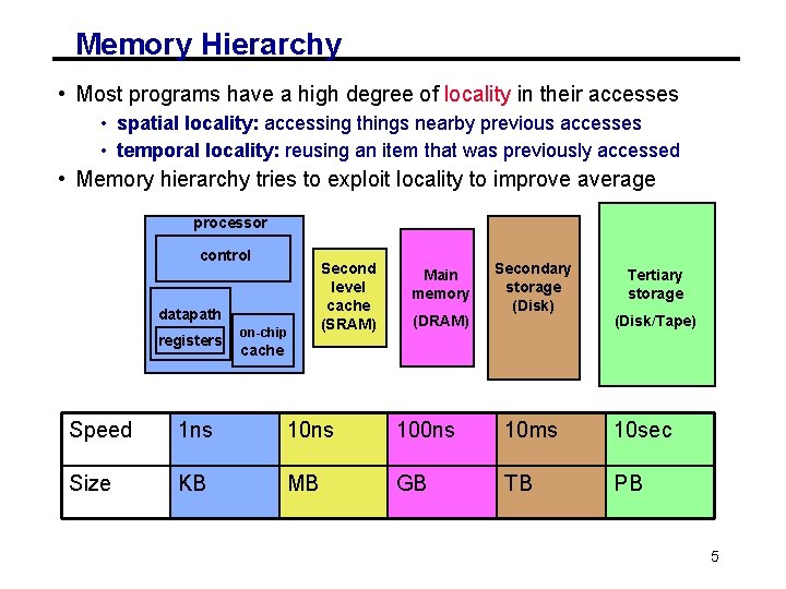
Memory Hierarchy • Most programs have a high degree of locality in their accesses • spatial locality: accessing things nearby previous accesses • temporal locality: reusing an item that was previously accessed • Memory hierarchy tries to exploit locality to improve average processor control datapath registers on-chip Second level cache (SRAM) Main memory (DRAM) Secondary storage (Disk) Tertiary storage (Disk/Tape) cache Speed 1 ns 100 ns 10 ms 10 sec Size KB MB GB TB PB 5

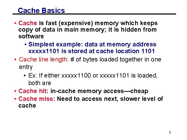
Cache Basics • Cache is fast (expensive) memory which keeps copy of data in main memory; it is hidden from software • Simplest example: data at memory address xxxxx 1101 is stored at cache location 1101 • Cache line length: # of bytes loaded together in one entry • Ex: If either xxxxx 1100 or xxxxx 1101 is loaded, both are • Cache hit: in-cache memory access—cheap • Cache miss: Need to access next, slower level of cache 6

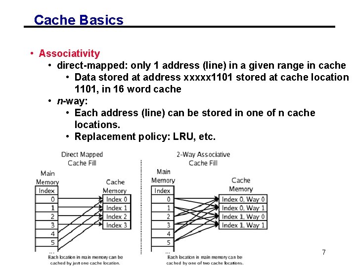
Cache Basics • Associativity • direct-mapped: only 1 address (line) in a given range in cache • Data stored at address xxxxx 1101 stored at cache location 1101, in 16 word cache • n-way: • Each address (line) can be stored in one of n cache locations. • Replacement policy: LRU, etc. 7

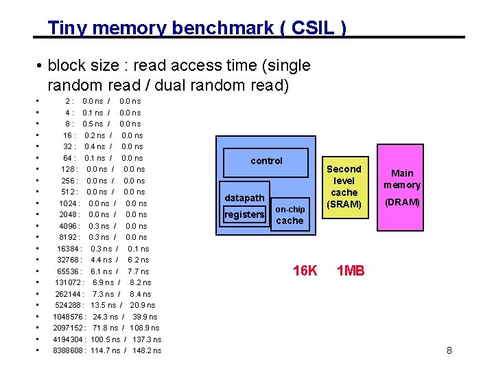
Tiny memory benchmark ( CSIL ) • block size : read access time (single random read / dual random read) • • • • • • 2 : 0. 0 ns / 0. 0 ns 4 : 0. 1 ns / 0. 0 ns 8 : 0. 5 ns / 0. 0 ns 16 : 0. 2 ns / 0. 0 ns 32 : 0. 4 ns / 0. 0 ns 64 : 0. 1 ns / 0. 0 ns 128 : 0. 0 ns / 0. 0 ns 256 : 0. 0 ns / 0. 0 ns 512 : 0. 0 ns / 0. 0 ns 1024 : 0. 0 ns / 0. 0 ns 2048 : 0. 0 ns / 0. 0 ns 4096 : 0. 3 ns / 0. 0 ns 8192 : 0. 3 ns / 0. 0 ns 16384 : 0. 3 ns / 0. 1 ns 32768 : 4. 4 ns / 6. 2 ns 65536 : 6. 1 ns / 7. 7 ns 131072 : 6. 9 ns / 8. 2 ns 262144 : 7. 3 ns / 8. 4 ns 524288 : 13. 5 ns / 20. 9 ns 1048576 : 24. 3 ns / 39. 9 ns 2097152 : 71. 8 ns / 108. 9 ns 4194304 : 100. 5 ns / 137. 3 ns 8388608 : 114. 7 ns / 148. 2 ns control datapath registers on-chip Second level cache (SRAM) Main memory (DRAM) cache 16 K 1 MB 8

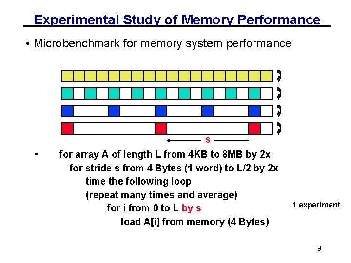
Experimental Study of Memory Performance • Microbenchmark for memory system performance s • for array A of length L from 4 KB to 8 MB by 2 x for stride s from 4 Bytes (1 word) to L/2 by 2 x time the following loop (repeat many times and average) for i from 0 to L by s load A[i] from memory (4 Bytes) 1 experiment 9

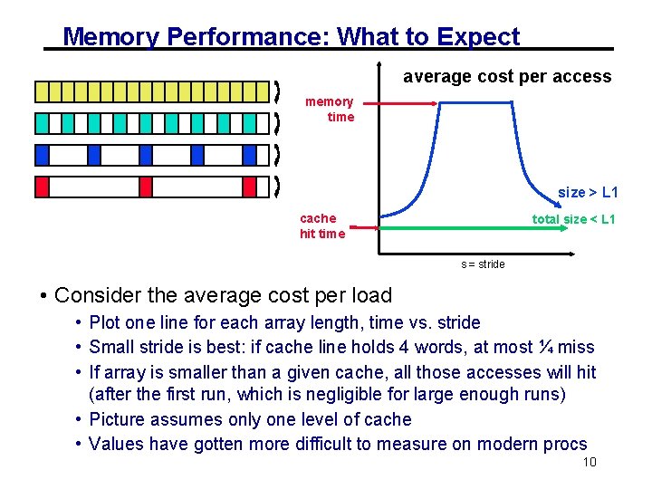
Memory Performance: What to Expect average cost per access memory time size > L 1 cache hit time total size < L 1 s = stride • Consider the average cost per load • Plot one line for each array length, time vs. stride • Small stride is best: if cache line holds 4 words, at most ¼ miss • If array is smaller than a given cache, all those accesses will hit (after the first run, which is negligible for large enough runs) • Picture assumes only one level of cache • Values have gotten more difficult to measure on modern procs 10

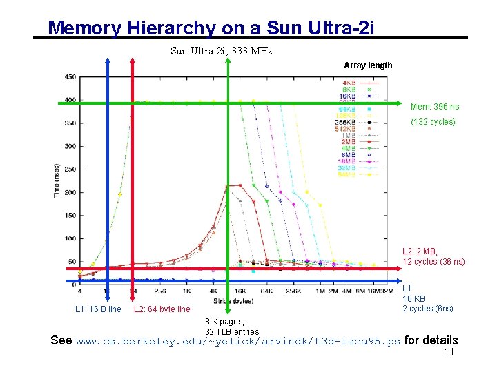
Memory Hierarchy on a Sun Ultra-2 i, 333 MHz Array length Mem: 396 ns (132 cycles) L 2: 2 MB, 12 cycles (36 ns) L 1: 16 B line L 1: 16 KB 2 cycles (6 ns) L 2: 64 byte line 8 K pages, 32 TLB entries See www. cs. berkeley. edu/~yelick/arvindk/t 3 d-isca 95. ps for details 11

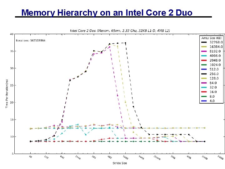
Memory Hierarchy on an Intel Core 2 Duo 12

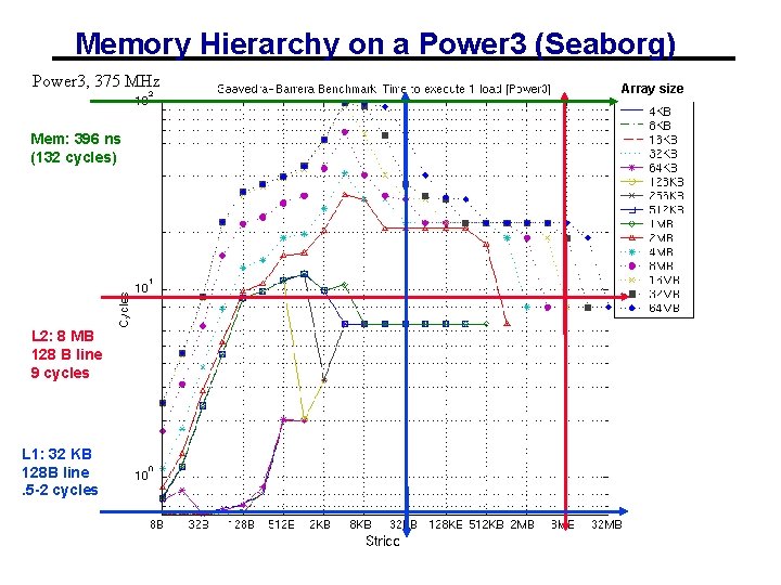
Memory Hierarchy on a Power 3 (Seaborg) Power 3, 375 MHz Array size Mem: 396 ns (132 cycles) L 2: 8 MB 128 B line 9 cycles L 1: 32 KB 128 B line. 5 -2 cycles 13

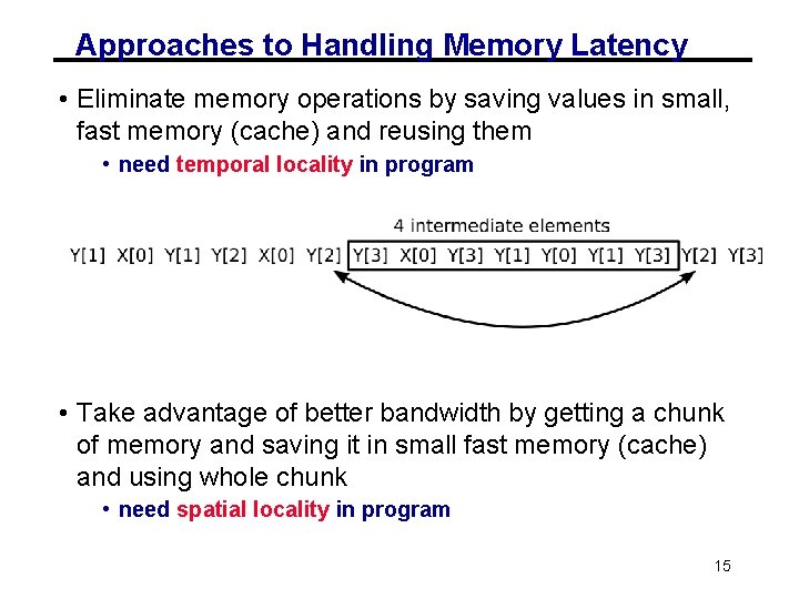
Approaches to Handling Memory Latency • Eliminate memory operations by saving values in small, fast memory (cache) and reusing them • need temporal locality in program • Take advantage of better bandwidth by getting a chunk of memory and saving it in small fast memory (cache) and using whole chunk • need spatial locality in program 15

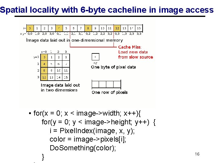
Spatial locality with 6 -byte cacheline in image access • for(x = 0; x < image->width; x++){ for(y = 0; y < image->height; y++) { i = Pixel. Index(image, x, y); color = image->pixels[i]; Do. Something(color); } 16

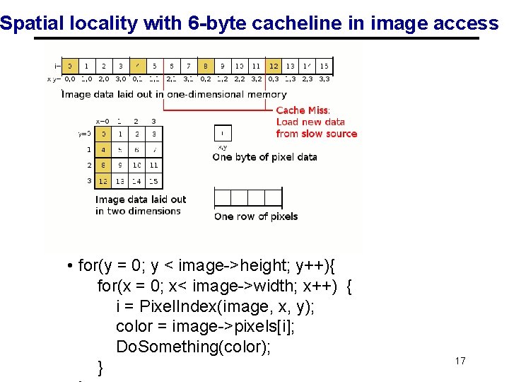
Spatial locality with 6 -byte cacheline in image access • for(y = 0; y < image->height; y++){ for(x = 0; x< image->width; x++) { i = Pixel. Index(image, x, y); color = image->pixels[i]; Do. Something(color); } 17

Other Approaches to Handling Memory Latency • Take advantage of better bandwidth by allowing processor to issue multiple reads to the memory system at once • concurrency in the instruction stream, e. g. load whole array, as in vector processors; or prefetching • Overlap computation & memory operations • prefetching 18

Lessons • Actual performance of a simple program can be a complicated function of the architecture • To write fast programs, need to consider architecture • True on sequential or parallel processor • Use simple models to help us design efficient algorithms • We will illustrate with a common technique for improving cache performance, called blocking or tiling • Organize data to fit in register/L 1 -cache/L 2 -cache 19

Outline • Idealized and actual costs in modern processors • Memory hierarchies • Use of microbenchmarks to characterized performance • Parallelism within a single processor • Case study: Matrix Multiplication • Use of performance models to optimize 20

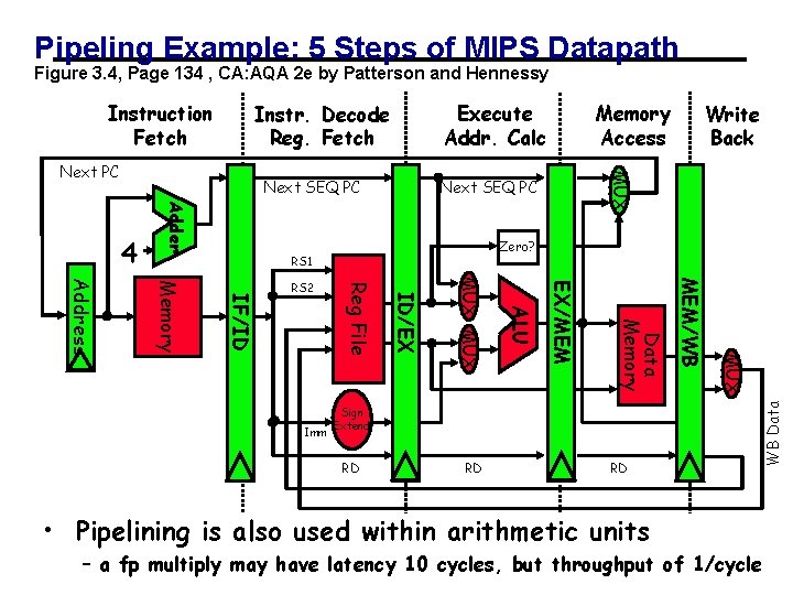
Pipeling Example: 5 Steps of MIPS Datapath Figure 3. 4, Page 134 , CA: AQA 2 e by Patterson and Hennessy Execute Addr. Calc Instr. Decode Reg. Fetch Next SEQ PC Adder 4 Zero? RS 1 RD RD RD • Pipelining is also used within arithmetic units MUX Sign Extend MEM/WB Data Memory EX/MEM ALU MUX ID/EX Imm Reg File IF/ID Memory Address RS 2 Write Back MUX Next PC Memory Access WB Data Instruction Fetch 21 – a fp multiply may have latency 10 cycles, but throughput of 1/cycle

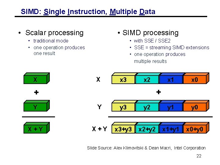
SIMD: Single Instruction, Multiple Data • Scalar processing • SIMD processing • traditional mode • one operation produces one result X • with SSE / SSE 2 • SSE = streaming SIMD extensions • one operation produces multiple results X x 3 x 2 x 1 x 0 + + Y Y y 3 y 2 y 1 y 0 X+Y x 3+y 3 x 2+y 2 x 1+y 1 x 0+y 0 Slide Source: Alex Klimovitski & Dean Macri, Intel Corporation 22

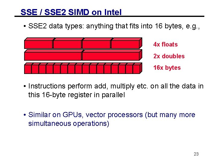
SSE / SSE 2 SIMD on Intel • SSE 2 data types: anything that fits into 16 bytes, e. g. , 4 x floats 2 x doubles 16 x bytes • Instructions perform add, multiply etc. on all the data in this 16 -byte register in parallel • Similar on GPUs, vector processors (but many more simultaneous operations) 23

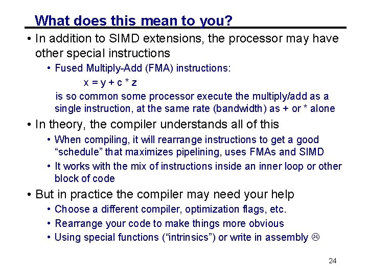
What does this mean to you? • In addition to SIMD extensions, the processor may have other special instructions • Fused Multiply-Add (FMA) instructions: x = y + c * z is so common some processor execute the multiply/add as a single instruction, at the same rate (bandwidth) as + or * alone • In theory, the compiler understands all of this • When compiling, it will rearrange instructions to get a good “schedule” that maximizes pipelining, uses FMAs and SIMD • It works with the mix of instructions inside an inner loop or other block of code • But in practice the compiler may need your help • Choose a different compiler, optimization flags, etc. • Rearrange your code to make things more obvious • Using special functions (“intrinsics”) or write in assembly 24

Outline • Idealized and actual costs in modern processors • Memory hierarchies • Use of microbenchmarks to characterized performance • Parallelism within single processors • Case study: Matrix Multiplication • Use of performance models to understand optimize performance 25

Case Study with Matrix Multiplication • An important kernel in many problems • Optimization ideas can be used in other problems • The most-studied algorithm in high performance computing • How to measure quality of implementation in terms of performance? • Megaflops number • Defined as: Core computation count / time spent • Matrix-matrix multiplication operation count = 2 n^3 • Example: 300 MFLOPS 300 million MM-related floating operations performed per second. 26

What do commercial and CSE applications have in common? (Red Hot Blue Cool)

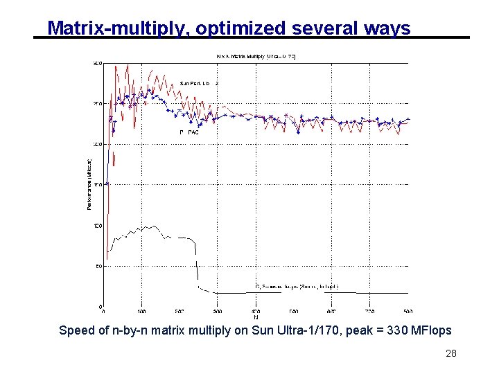
Matrix-multiply, optimized several ways Speed of n-by-n matrix multiply on Sun Ultra-1/170, peak = 330 MFlops 28

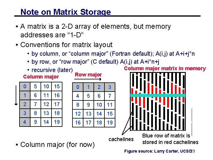
Note on Matrix Storage • A matrix is a 2 -D array of elements, but memory addresses are “ 1 -D” • Conventions for matrix layout • by column, or “column major” (Fortran default); A(i, j) at A+i+j*n • by row, or “row major” (C default) A(i, j) at A+i*n+j Column major matrix in memory • recursive (later) Column major Row major 0 5 10 15 0 1 2 3 1 6 11 16 4 5 6 7 2 7 12 17 8 9 10 11 3 8 13 18 12 13 14 15 4 9 14 19 16 17 18 19 • Column major (for now) cachelines Blue row of matrix is stored in red cachelines Figure source: Larry Carter, UCSD 29

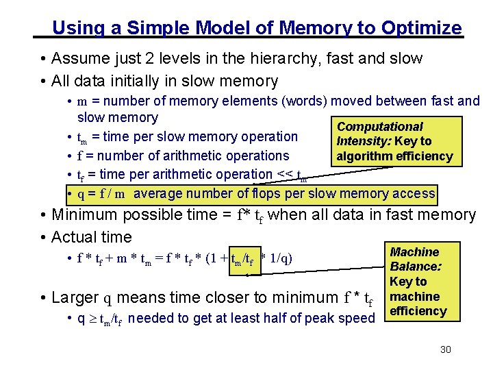
Using a Simple Model of Memory to Optimize • Assume just 2 levels in the hierarchy, fast and slow • All data initially in slow memory • m = number of memory elements (words) moved between fast and slow memory Computational • tm = time per slow memory operation Intensity: Key to • f = number of arithmetic operations algorithm efficiency • tf = time per arithmetic operation << tm • q = f / m average number of flops per slow memory access • Minimum possible time = f* tf when all data in fast memory • Actual time • f * tf + m * tm = f * tf * (1 + tm/tf * 1/q) • Larger q means time closer to minimum f * tf • q tm/tf needed to get at least half of peak speed Machine Balance: Key to machine efficiency 30

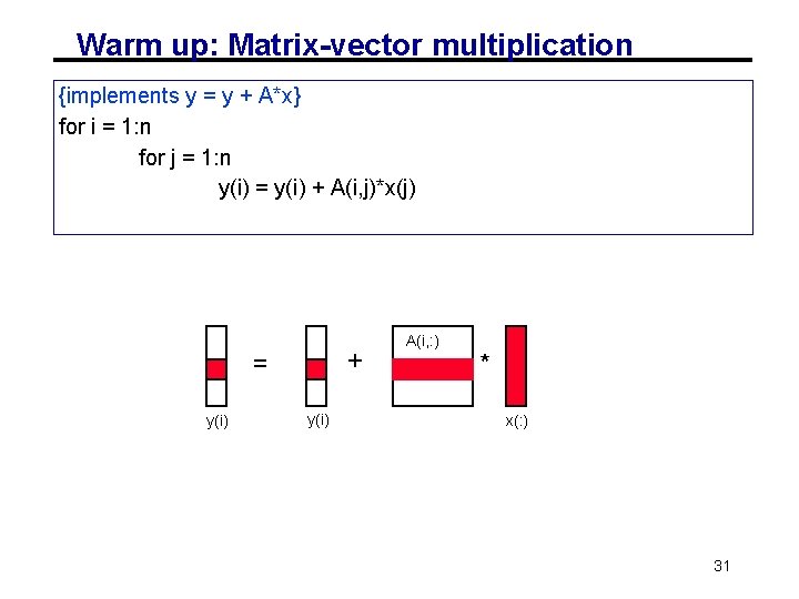
Warm up: Matrix-vector multiplication {implements y = y + A*x} for i = 1: n for j = 1: n y(i) = y(i) + A(i, j)*x(j) + = y(i) A(i, : ) * x(: ) 31

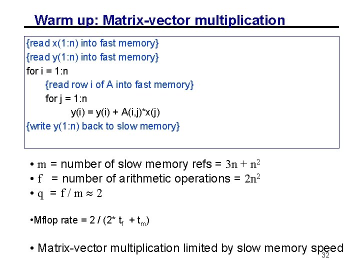
Warm up: Matrix-vector multiplication {read x(1: n) into fast memory} {read y(1: n) into fast memory} for i = 1: n {read row i of A into fast memory} for j = 1: n y(i) = y(i) + A(i, j)*x(j) {write y(1: n) back to slow memory} • m = number of slow memory refs = 3 n + n 2 • f = number of arithmetic operations = 2 n 2 • q = f / m 2 • Mflop rate = 2 / (2* tf + tm) • Matrix-vector multiplication limited by slow memory speed 32

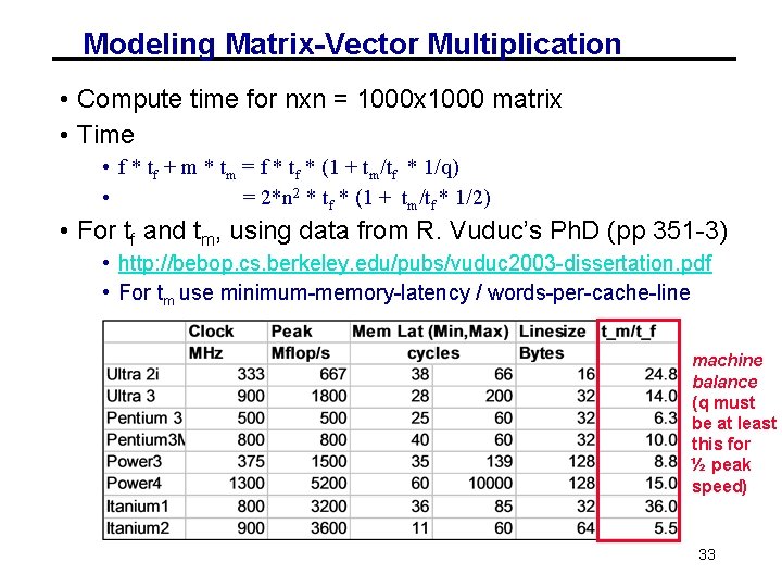
Modeling Matrix-Vector Multiplication • Compute time for nxn = 1000 x 1000 matrix • Time • f * tf + m * tm = f * tf * (1 + tm/tf * 1/q) • = 2*n 2 * tf * (1 + tm/tf * 1/2) • For tf and tm, using data from R. Vuduc’s Ph. D (pp 351 -3) • http: //bebop. cs. berkeley. edu/pubs/vuduc 2003 -dissertation. pdf • For tm use minimum-memory-latency / words-per-cache-line machine balance (q must be at least this for ½ peak speed) 33

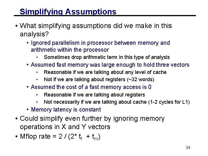
Simplifying Assumptions • What simplifying assumptions did we make in this analysis? • Ignored parallelism in processor between memory and arithmetic within the processor • Sometimes drop arithmetic term in this type of analysis • Assumed fast memory was large enough to hold three vectors • • Reasonable if we are talking about any level of cache Not if we are talking about registers (~32 words) • Assumed the cost of a fast memory access is 0 • • Reasonable if we are talking about registers Not necessarily if we are talking about cache (1 -2 cycles for L 1) • Memory latency is constant • Could simplify even further by ignoring memory operations in X and Y vectors • Mflop rate = 2 / (2* tf + tm) 34

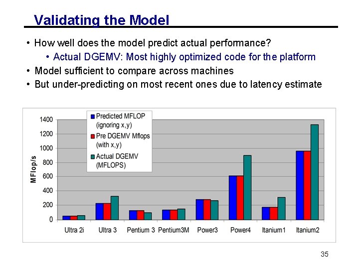
Validating the Model • How well does the model predict actual performance? • Actual DGEMV: Most highly optimized code for the platform • Model sufficient to compare across machines • But under-predicting on most recent ones due to latency estimate 35

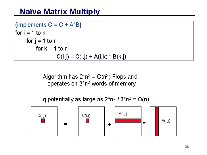
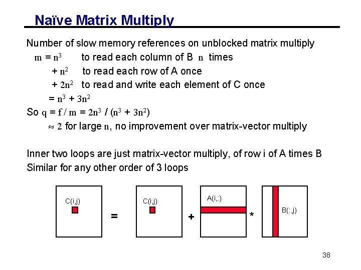
Naïve Matrix Multiply {implements C = C + A*B} for i = 1 to n for j = 1 to n for k = 1 to n C(i, j) = C(i, j) + A(i, k) * B(k, j) Algorithm has 2*n 3 = O(n 3) Flops and operates on 3*n 2 words of memory q potentially as large as 2*n 3 / 3*n 2 = O(n) C(i, j) A(i, : ) C(i, j) = + * B(: , j) 36

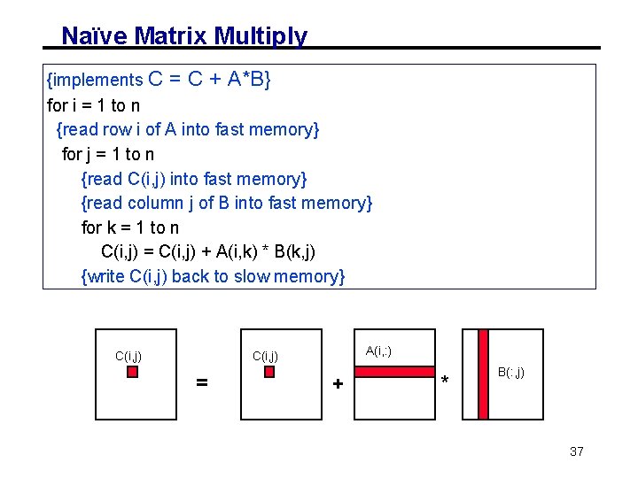
Naïve Matrix Multiply {implements C = C + A*B} for i = 1 to n {read row i of A into fast memory} for j = 1 to n {read C(i, j) into fast memory} {read column j of B into fast memory} for k = 1 to n C(i, j) = C(i, j) + A(i, k) * B(k, j) {write C(i, j) back to slow memory} C(i, j) A(i, : ) C(i, j) = + * B(: , j) 37

Naïve Matrix Multiply Number of slow memory references on unblocked matrix multiply m = n 3 to read each column of B n times + n 2 to read each row of A once + 2 n 2 to read and write each element of C once = n 3 + 3 n 2 So q = f / m = 2 n 3 / (n 3 + 3 n 2) 2 for large n, no improvement over matrix-vector multiply Inner two loops are just matrix-vector multiply, of row i of A times B Similar for any other order of 3 loops C(i, j) A(i, : ) C(i, j) = + * B(: , j) 38

Matrix-multiply, optimized several ways Speed of n-by-n matrix multiply on Sun Ultra-1/170, peak = 330 MFlops 39

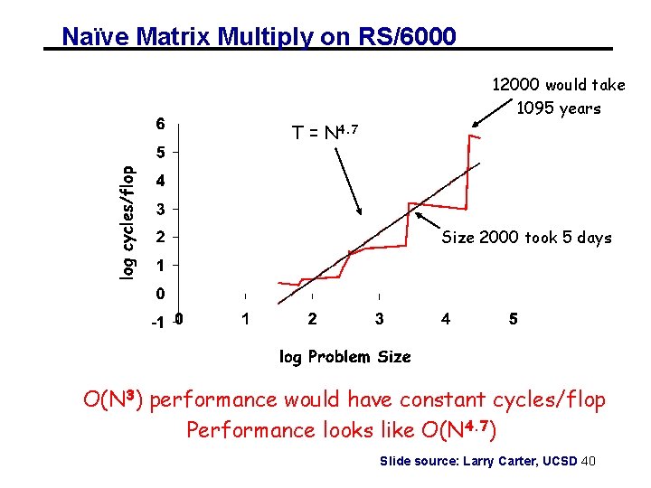
Naïve Matrix Multiply on RS/6000 12000 would take 1095 years T = N 4. 7 Size 2000 took 5 days O(N 3) performance would have constant cycles/flop Performance looks like O(N 4. 7) Slide source: Larry Carter, UCSD 40

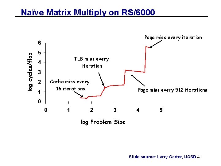
Naïve Matrix Multiply on RS/6000 Page miss every iteration TLB miss every iteration Cache miss every 16 iterations Page miss every 512 iterations Slide source: Larry Carter, UCSD 41

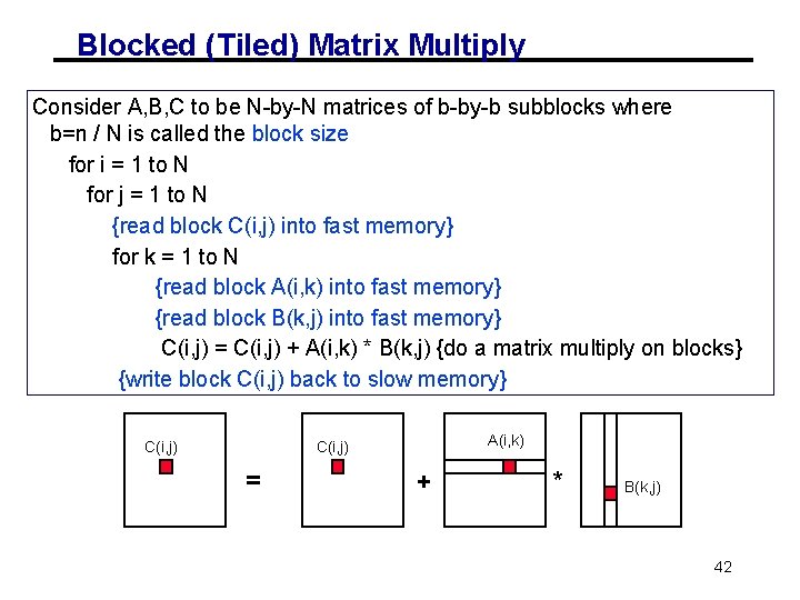
Blocked (Tiled) Matrix Multiply Consider A, B, C to be N-by-N matrices of b-by-b subblocks where b=n / N is called the block size for i = 1 to N for j = 1 to N {read block C(i, j) into fast memory} for k = 1 to N {read block A(i, k) into fast memory} {read block B(k, j) into fast memory} C(i, j) = C(i, j) + A(i, k) * B(k, j) {do a matrix multiply on blocks} {write block C(i, j) back to slow memory} C(i, j) A(i, k) C(i, j) = + * B(k, j) 42

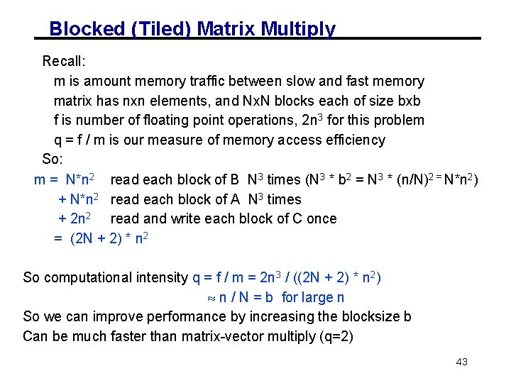
Blocked (Tiled) Matrix Multiply Recall: m is amount memory traffic between slow and fast memory matrix has nxn elements, and Nx. N blocks each of size bxb f is number of floating point operations, 2 n 3 for this problem q = f / m is our measure of memory access efficiency So: m = N*n 2 read each block of B N 3 times (N 3 * b 2 = N 3 * (n/N)2 = N*n 2) + N*n 2 read each block of A N 3 times + 2 n 2 read and write each block of C once = (2 N + 2) * n 2 So computational intensity q = f / m = 2 n 3 / ((2 N + 2) * n 2) n / N = b for large n So we can improve performance by increasing the blocksize b Can be much faster than matrix-vector multiply (q=2) 43

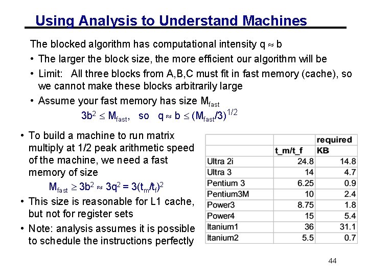
Using Analysis to Understand Machines The blocked algorithm has computational intensity q b • The larger the block size, the more efficient our algorithm will be • Limit: All three blocks from A, B, C must fit in fast memory (cache), so we cannot make these blocks arbitrarily large • Assume your fast memory has size Mfast 3 b 2 Mfast, so q b (Mfast/3)1/2 • To build a machine to run matrix multiply at 1/2 peak arithmetic speed of the machine, we need a fast memory of size Mfast 3 b 2 3 q 2 = 3(tm/tf)2 • This size is reasonable for L 1 cache, but not for register sets • Note: analysis assumes it is possible to schedule the instructions perfectly 44

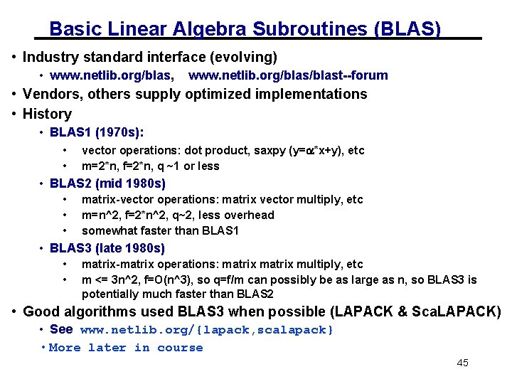
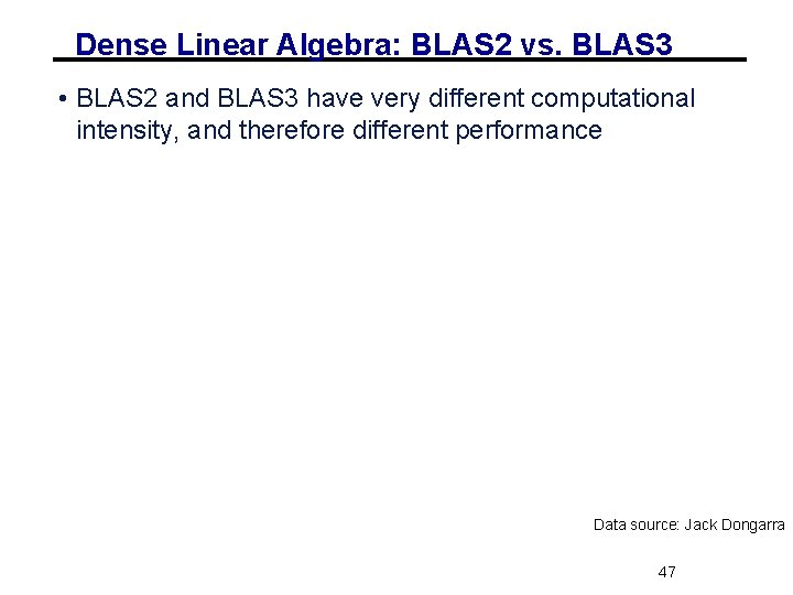
Basic Linear Algebra Subroutines (BLAS) • Industry standard interface (evolving) • www. netlib. org/blas, www. netlib. org/blast--forum • Vendors, others supply optimized implementations • History • BLAS 1 (1970 s): • • vector operations: dot product, saxpy (y=a*x+y), etc m=2*n, f=2*n, q ~1 or less • BLAS 2 (mid 1980 s) • • • matrix-vector operations: matrix vector multiply, etc m=n^2, f=2*n^2, q~2, less overhead somewhat faster than BLAS 1 • BLAS 3 (late 1980 s) • • matrix-matrix operations: matrix multiply, etc m <= 3 n^2, f=O(n^3), so q=f/m can possibly be as large as n, so BLAS 3 is potentially much faster than BLAS 2 • Good algorithms used BLAS 3 when possible (LAPACK & Sca. LAPACK) • See www. netlib. org/{lapack, scalapack} • More later in course 45

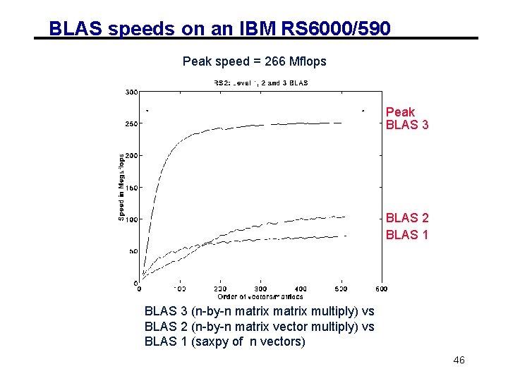
BLAS speeds on an IBM RS 6000/590 Peak speed = 266 Mflops Peak BLAS 3 BLAS 2 BLAS 1 BLAS 3 (n-by-n matrix multiply) vs BLAS 2 (n-by-n matrix vector multiply) vs BLAS 1 (saxpy of n vectors) 46

Dense Linear Algebra: BLAS 2 vs. BLAS 3 • BLAS 2 and BLAS 3 have very different computational intensity, and therefore different performance Data source: Jack Dongarra 47

Search Over Block Sizes • Performance models are useful for high level algorithms • Helps in developing a blocked algorithm • Models have not proven very useful for block size selection • too complicated to be useful – See work by Sid Chatterjee for detailed model • too simple to be accurate – Multiple multidimensional arrays, virtual memory, etc. • Speed depends on matrix dimensions, details of code, compiler, processor 48

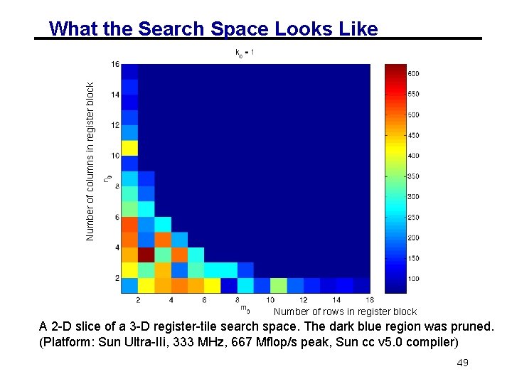
Number of columns in register block What the Search Space Looks Like Number of rows in register block A 2 -D slice of a 3 -D register-tile search space. The dark blue region was pruned. (Platform: Sun Ultra-IIi, 333 MHz, 667 Mflop/s peak, Sun cc v 5. 0 compiler) 49

Optimizing Code in Practice • Tiling for registers • loop unrolling, use of named “register” variables • Tiling for multiple levels of cache and TLB • Exploiting fine-grained parallelism in processor • superscalar; pipelining • Complicated compiler interactions • Hard to do by hand (but you’ll try) • Automatic optimization an active research area 50

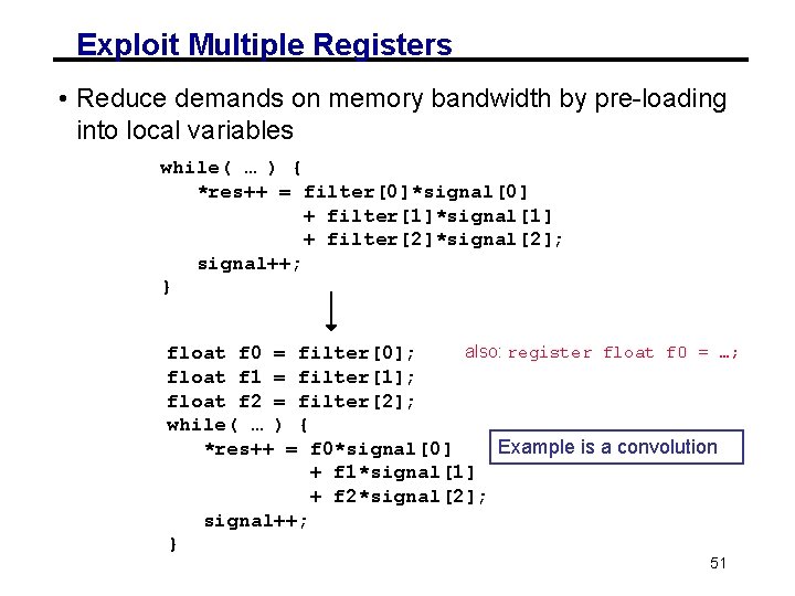
Exploit Multiple Registers • Reduce demands on memory bandwidth by pre-loading into local variables while( … ) { *res++ = filter[0]*signal[0] + filter[1]*signal[1] + filter[2]*signal[2]; signal++; } also: register float f 0 = …; float f 0 = filter[0]; float f 1 = filter[1]; float f 2 = filter[2]; while( … ) { Example is a convolution *res++ = f 0*signal[0] + f 1*signal[1] + f 2*signal[2]; signal++; } 51

Loop Unrolling • Expose instruction-level parallelism float f 0 = filter[0], f 1 = filter[1], f 2 = filter[2]; float s 0 = signal[0], s 1 = signal[1], s 2 = signal[2]; *res++ = f 0*s 0 + f 1*s 1 + f 2*s 2; do { signal += 3; s 0 = signal[0]; res[0] = f 0*s 1 + f 1*s 2 + f 2*s 0; s 1 = signal[1]; res[1] = f 0*s 2 + f 1*s 0 + f 2*s 1; s 2 = signal[2]; res[2] = f 0*s 0 + f 1*s 1 + f 2*s 2; res += 3; } while( … ); 53

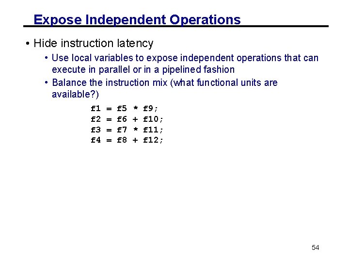
Expose Independent Operations • Hide instruction latency • Use local variables to expose independent operations that can execute in parallel or in a pipelined fashion • Balance the instruction mix (what functional units are available? ) f 1 f 2 f 3 f 4 = = f 5 f 6 f 7 f 8 * + f 9; f 10; f 11; f 12; 54

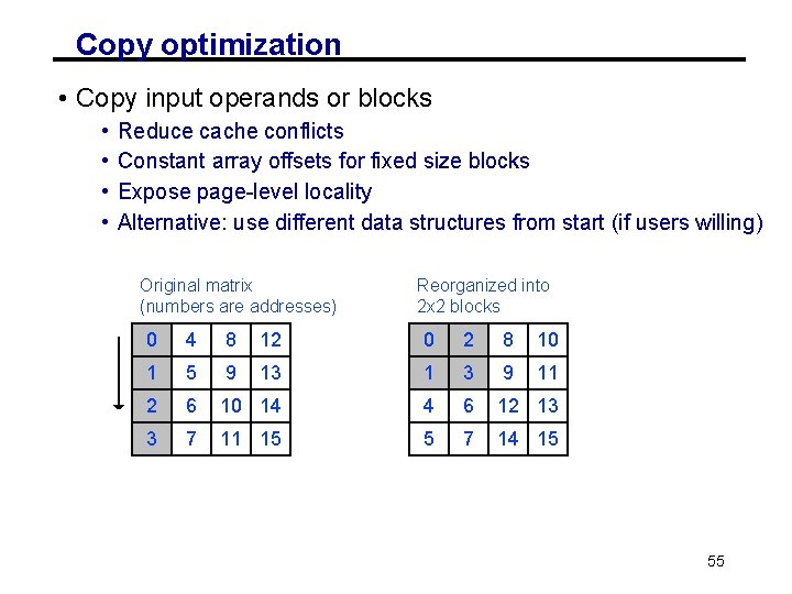
Copy optimization • Copy input operands or blocks • • Reduce cache conflicts Constant array offsets for fixed size blocks Expose page-level locality Alternative: use different data structures from start (if users willing) Original matrix (numbers are addresses) Reorganized into 2 x 2 blocks 0 4 8 12 0 2 8 10 1 5 9 13 1 3 9 11 2 6 10 14 4 6 12 13 3 7 11 15 5 7 14 15 55

Questions You Should Be Able to Answer 1. What is the key to understand algorithm efficiency in our simple memory model? 2. What is tiling? 3. Why does block matrix multiply reduce the number of memory references? 4. What are the BLAS? 5. Why does loop unrolling improve uniprocessor performance? 57

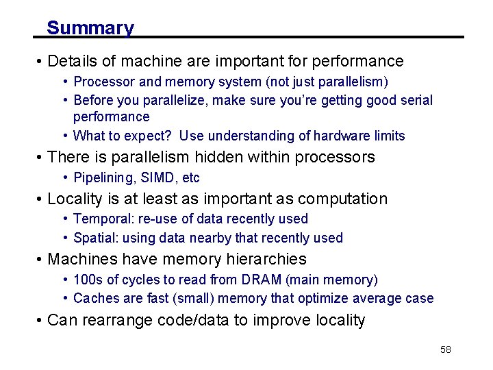
Summary • Details of machine are important for performance • Processor and memory system (not just parallelism) • Before you parallelize, make sure you’re getting good serial performance • What to expect? Use understanding of hardware limits • There is parallelism hidden within processors • Pipelining, SIMD, etc • Locality is at least as important as computation • Temporal: re-use of data recently used • Spatial: using data nearby that recently used • Machines have memory hierarchies • 100 s of cycles to read from DRAM (main memory) • Caches are fast (small) memory that optimize average case • Can rearrange code/data to improve locality 58