Computer aided design CAD with Aspen Plus Javad

Computer aided design (CAD) with Aspen Plus Javad Ahmadpour j. ahmadpour@nit. ac. ir 1

THE OPTIMIZATION TOOL Using Aspen Plus® V 9. 0

PROBLEM DESCRIPTION: DEFINING THE OBJECTIVE FUNCTION • As quoted from Peters and Timmerhaus [1]: “Piping is a major item in the cost of chemical process plants. These costs in a fluid-process plant can run as high as 80% of the purchased equipment cost or 20% of the fixed capital investment”. • The diameter of the pipe strongly influences the present value of the plant, through both the annual cost of electric power and the installation cost of the piping system (pipe, pumps, valves, etc. ). • In this chapter, we expand the work and give a more precise and detailed model on how to find the optimum diameter under turbulent condition.

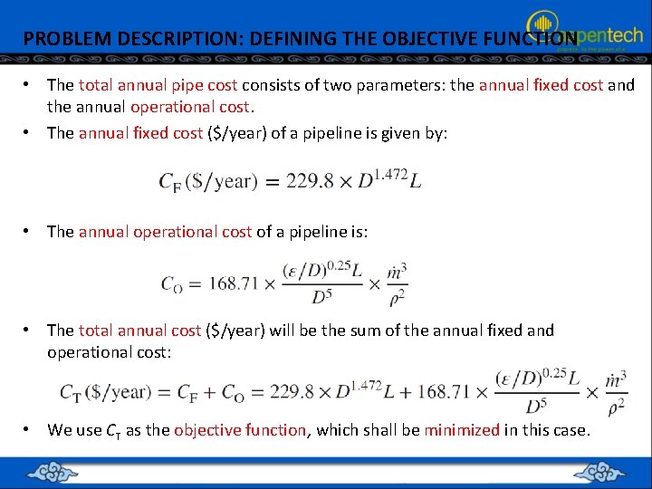
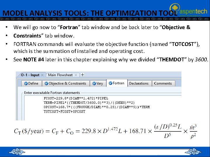
PROBLEM DESCRIPTION: DEFINING THE OBJECTIVE FUNCTION • The total annual pipe cost consists of two parameters: the annual fixed cost and the annual operational cost. • The annual fixed cost ($/year) of a pipeline is given by: • The annual operational cost of a pipeline is: • The total annual cost ($/year) will be the sum of the annual fixed and operational cost: • We use CT as the objective function, which shall be minimized in this case.

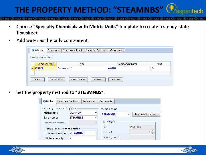
THE PROPERTY METHOD: “STEAMNBS” • Choose “Specialty Chemicals with Metric Units” template to create a steady-state flowsheet. Add water as the only component. • Set the property method to “STEAMNBS”. •

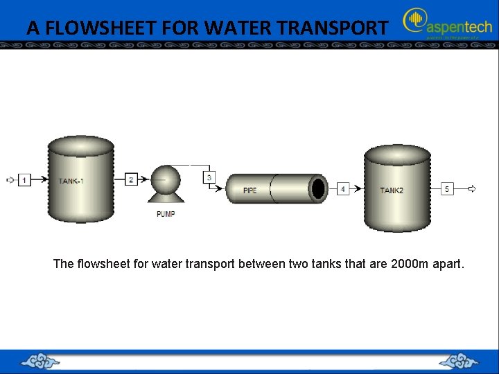
A FLOWSHEET FOR WATER TRANSPORT The flowsheet for water transport between two tanks that are 2000 m apart.

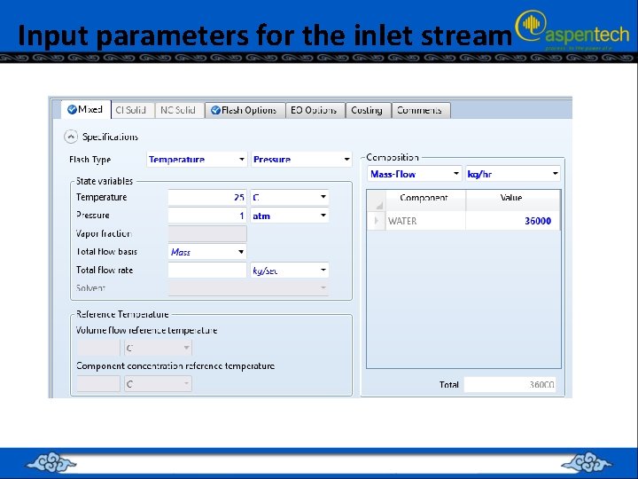
Input parameters for the inlet stream

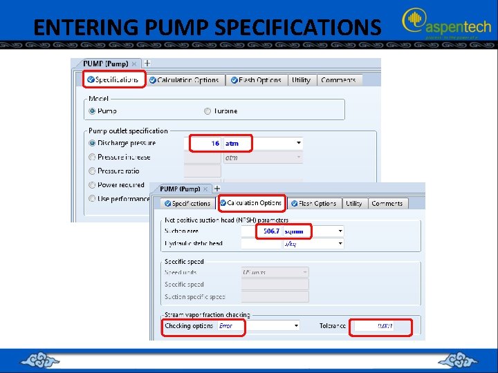
ENTERING PUMP SPECIFICATIONS

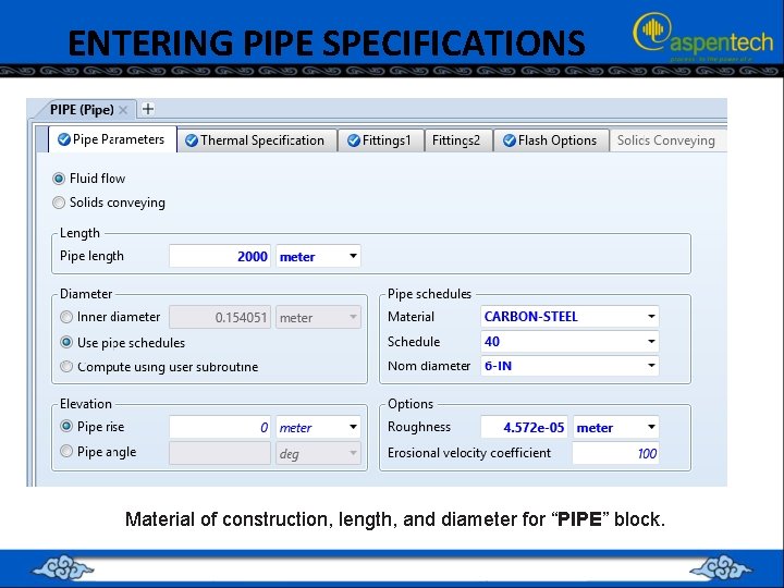
ENTERING PIPE SPECIFICATIONS Material of construction, length, and diameter for “PIPE” block.

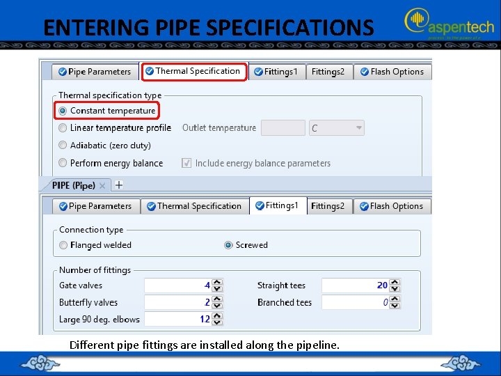
ENTERING PIPE SPECIFICATIONS Different pipe fittings are installed along the pipeline.

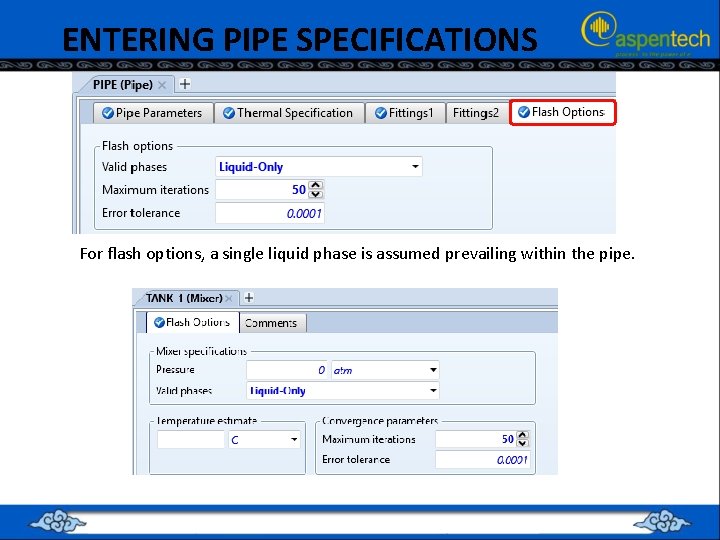
ENTERING PIPE SPECIFICATIONS For flash options, a single liquid phase is assumed prevailing within the pipe.

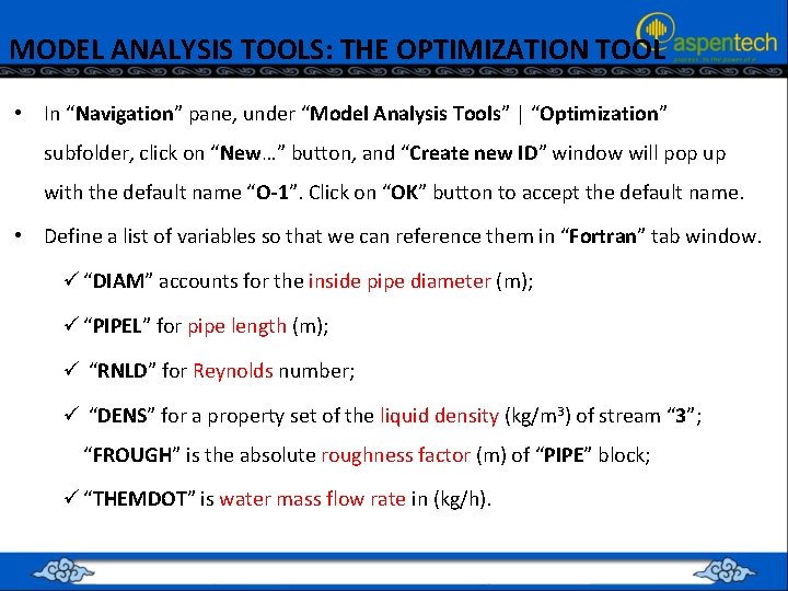
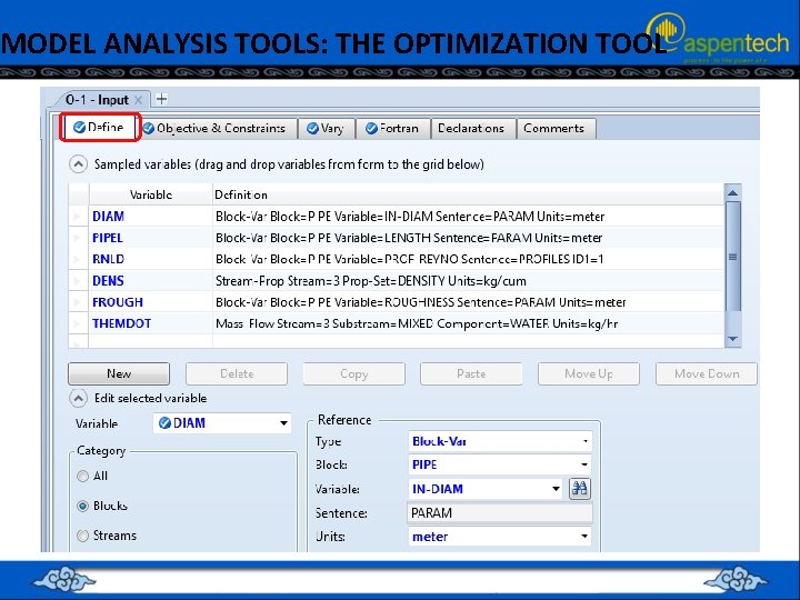
MODEL ANALYSIS TOOLS: THE OPTIMIZATION TOOL • In “Navigation” pane, under “Model Analysis Tools” | “Optimization” subfolder, click on “New…” button, and “Create new ID” window will pop up with the default name “O-1”. Click on “OK” button to accept the default name. • Define a list of variables so that we can reference them in “Fortran” tab window. ü “DIAM” accounts for the inside pipe diameter (m); ü “PIPEL” for pipe length (m); ü “RNLD” for Reynolds number; ü “DENS” for a property set of the liquid density (kg/m 3) of stream “ 3”; “FROUGH” is the absolute roughness factor (m) of “PIPE” block; ü “THEMDOT” is water mass flow rate in (kg/h).

MODEL ANALYSIS TOOLS: THE OPTIMIZATION TOOL

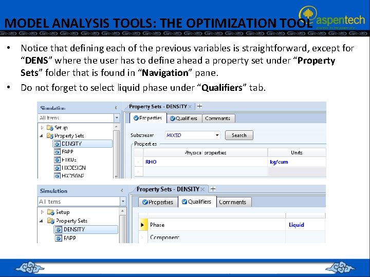
MODEL ANALYSIS TOOLS: THE OPTIMIZATION TOOL • Notice that defining each of the previous variables is straightforward, except for “DENS” where the user has to define ahead a property set under “Property Sets” folder that is found in “Navigation” pane. • Do not forget to select liquid phase under “Qualifiers” tab.

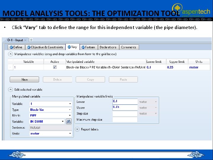
MODEL ANALYSIS TOOLS: THE OPTIMIZATION TOOL • Click “Vary” tab to define the range for this independent variable (the pipe diameter).

MODEL ANALYSIS TOOLS: THE OPTIMIZATION TOOL • We will go now to “Fortran” tab window and be back later to “Objective & • Constraints” tab window. • FORTRAN commands will evaluate the objective function (named “TOTCOST”), which is the summation of installed and operating cost. • See NOTE #4 later in this chapter explaining why we divided “THEMDOT” by 3600.

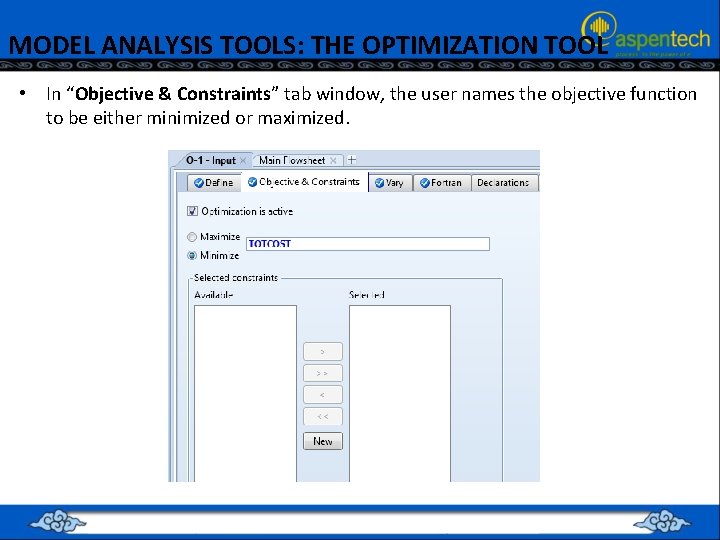
MODEL ANALYSIS TOOLS: THE OPTIMIZATION TOOL • In “Objective & Constraints” tab window, the user names the objective function to be either minimized or maximized.

MODEL ANALYSIS TOOLS: THE OPTIMIZATION TOOL

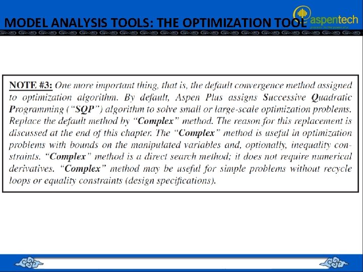
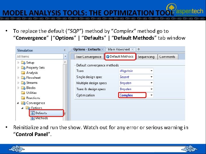
MODEL ANALYSIS TOOLS: THE OPTIMIZATION TOOL • To replace the default (“SQP”) method by “Complex” method go to “Convergence” |“Options” | “Default Methods” tab window • Reinitialize and run the show. Watch out for any error or serious warning in “Control Panel”.

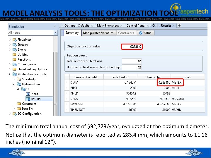
MODEL ANALYSIS TOOLS: THE OPTIMIZATION TOOL The minimum total annual cost of $92, 729/year, evaluated at the optimum diameter. Notice that the optimum diameter is reported as 283. 4 mm, which amounts to 11. 16 inches (nominal 12′′).

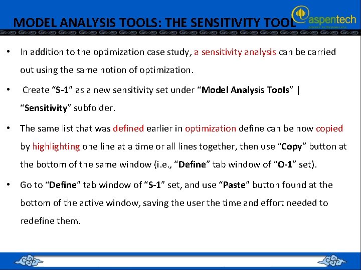
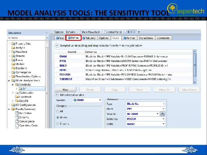
MODEL ANALYSIS TOOLS: THE SENSITIVITY TOOL • In addition to the optimization case study, a sensitivity analysis can be carried out using the same notion of optimization. • Create “S-1” as a new sensitivity set under “Model Analysis Tools” | “Sensitivity” subfolder. • The same list that was defined earlier in optimization define can be now copied by highlighting one line at a time or all lines together, then use “Copy” button at the bottom of the same window (i. e. , “Define” tab window of “O-1” set). • Go to “Define” tab window of “S-1” set, and use “Paste” button found at the bottom of the active window, saving the user the time and effort needed to redefine them.

MODEL ANALYSIS TOOLS: THE SENSITIVITY TOOL

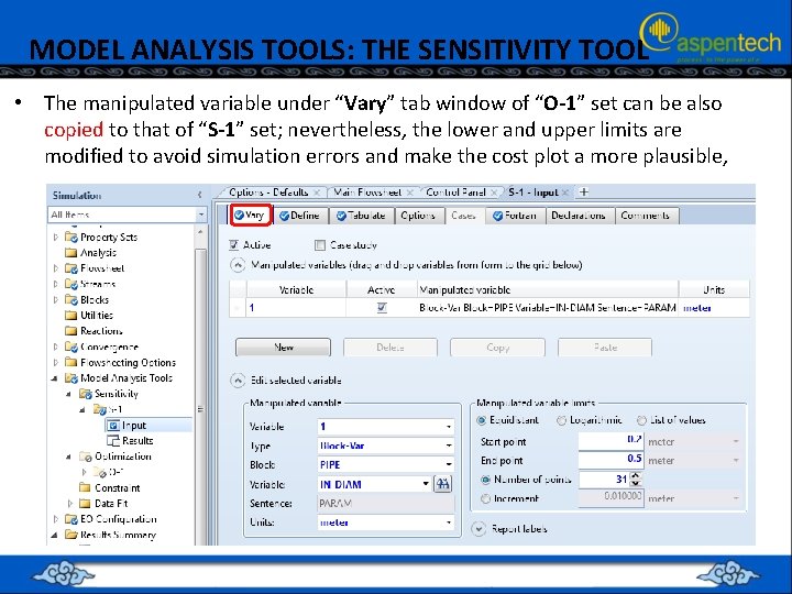
MODEL ANALYSIS TOOLS: THE SENSITIVITY TOOL • The manipulated variable under “Vary” tab window of “O-1” set can be also copied to that of “S-1” set; nevertheless, the lower and upper limits are modified to avoid simulation errors and make the cost plot a more plausible,

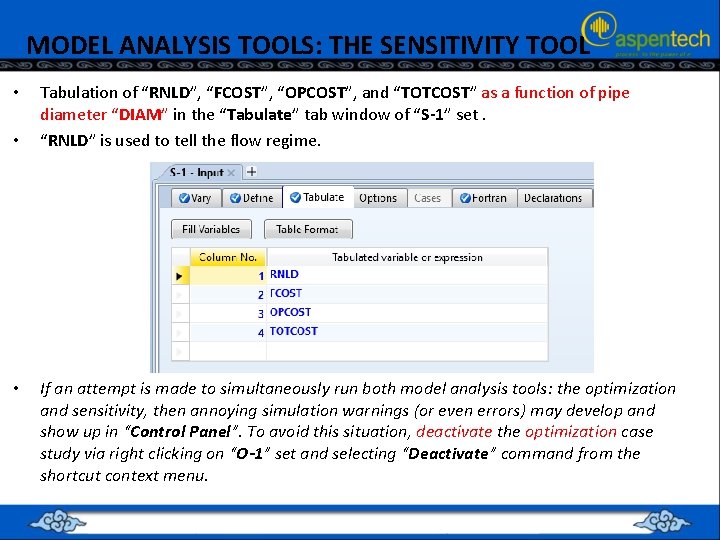
MODEL ANALYSIS TOOLS: THE SENSITIVITY TOOL • • • Tabulation of “RNLD”, “FCOST”, “OPCOST”, and “TOTCOST” as a function of pipe diameter “DIAM” in the “Tabulate” tab window of “S-1” set. “RNLD” is used to tell the flow regime. If an attempt is made to simultaneously run both model analysis tools: the optimization and sensitivity, then annoying simulation warnings (or even errors) may develop and show up in “Control Panel”. To avoid this situation, deactivate the optimization case study via right clicking on “O-1” set and selecting “Deactivate” command from the shortcut context menu.

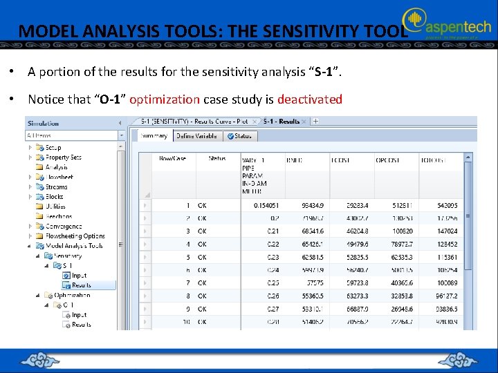
MODEL ANALYSIS TOOLS: THE SENSITIVITY TOOL • A portion of the results for the sensitivity analysis “S-1”. • Notice that “O-1” optimization case study is deactivated

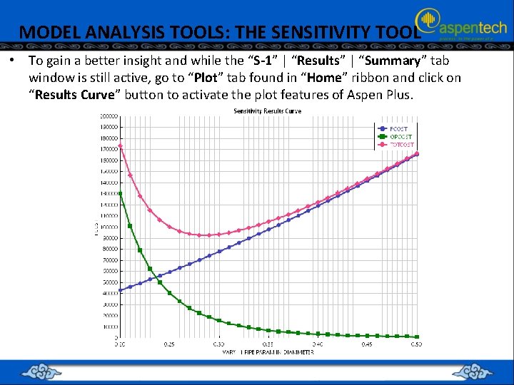
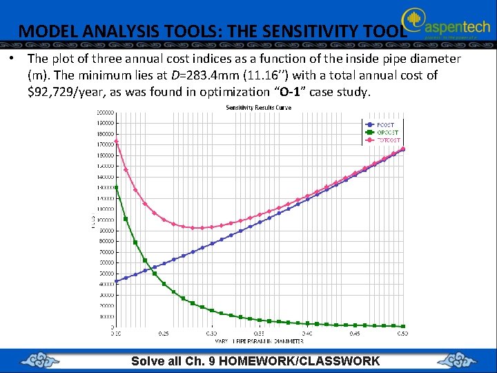
MODEL ANALYSIS TOOLS: THE SENSITIVITY TOOL • To gain a better insight and while the “S-1” | “Results” | “Summary” tab window is still active, go to “Plot” tab found in “Home” ribbon and click on “Results Curve” button to activate the plot features of Aspen Plus.

MODEL ANALYSIS TOOLS: THE SENSITIVITY TOOL • The plot of three annual cost indices as a function of the inside pipe diameter (m). The minimum lies at D=283. 4 mm (11. 16′′) with a total annual cost of $92, 729/year, as was found in optimization “O-1” case study. Solve all Ch. 9 HOMEWORK/CLASSWORK

DISTILLATION ECONOMIC OPTIMIZATION Using Aspen Plus® V 9. 0

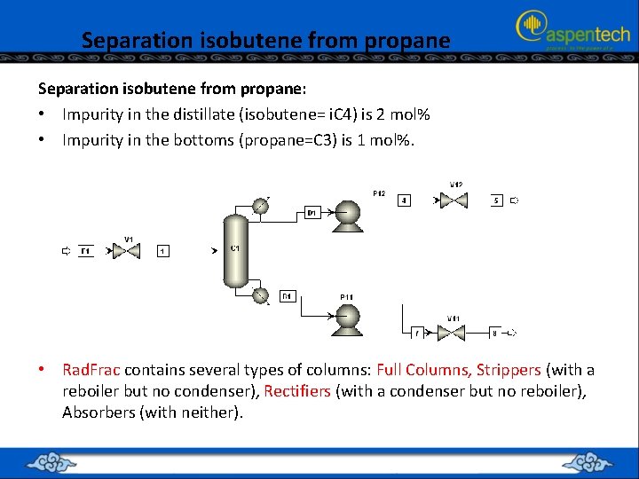
Separation isobutene from propane: • Impurity in the distillate (isobutene= i. C 4) is 2 mol% • Impurity in the bottoms (propane=C 3) is 1 mol%. • Rad. Frac contains several types of columns: Full Columns, Strippers (with a reboiler but no condenser), Rectifiers (with a condenser but no reboiler), Absorbers (with neither).

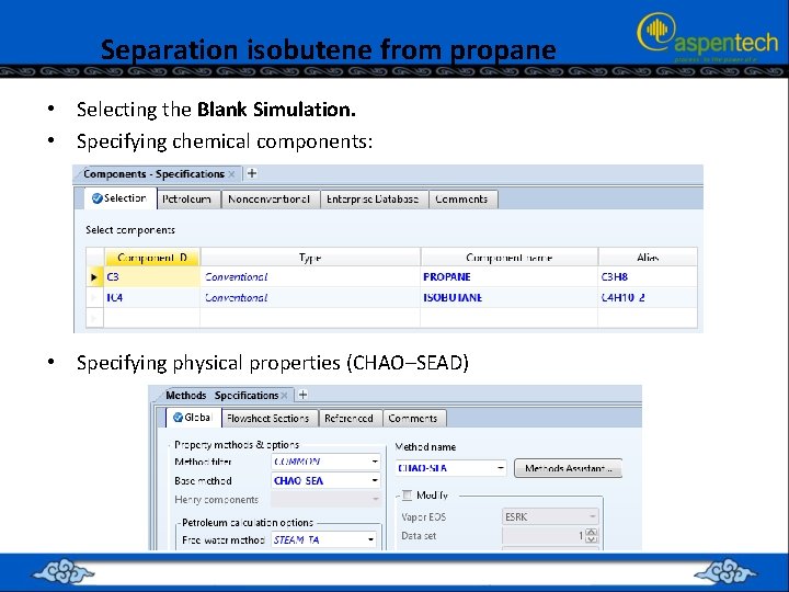
Separation isobutene from propane • Selecting the Blank Simulation. • Specifying chemical components: • Specifying physical properties (CHAO–SEAD)

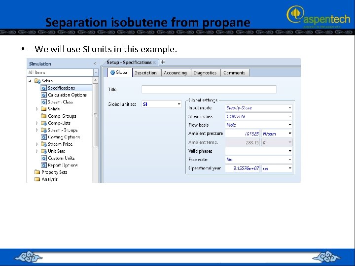
Separation isobutene from propane • We will use SI units in this example.

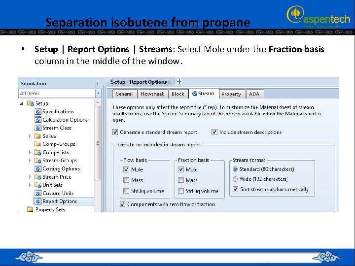
Separation isobutene from propane • Setup | Report Options | Streams: Select Mole under the Fraction basis column in the middle of the window.

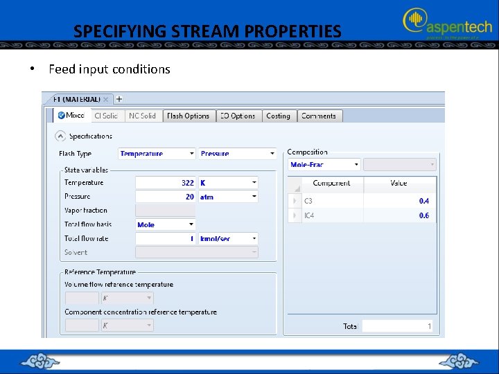
SPECIFYING STREAM PROPERTIES • Feed input conditions

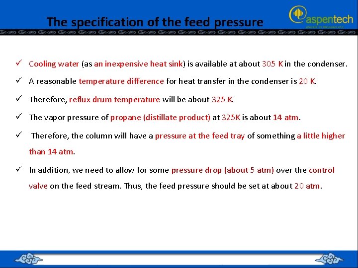
The specification of the feed pressure ü Cooling water (as an inexpensive heat sink) is available at about 305 K in the condenser. ü A reasonable temperature difference for heat transfer in the condenser is 20 K. ü Therefore, reflux drum temperature will be about 325 K. ü The vapor pressure of propane (distillate product) at 325 K is about 14 atm. ü Therefore, the column will have a pressure at the feed tray of something a little higher than 14 atm. ü In addition, we need to allow for some pressure drop (about 5 atm) over the control valve on the feed stream. Thus, the feed pressure should be set at about 20 atm.

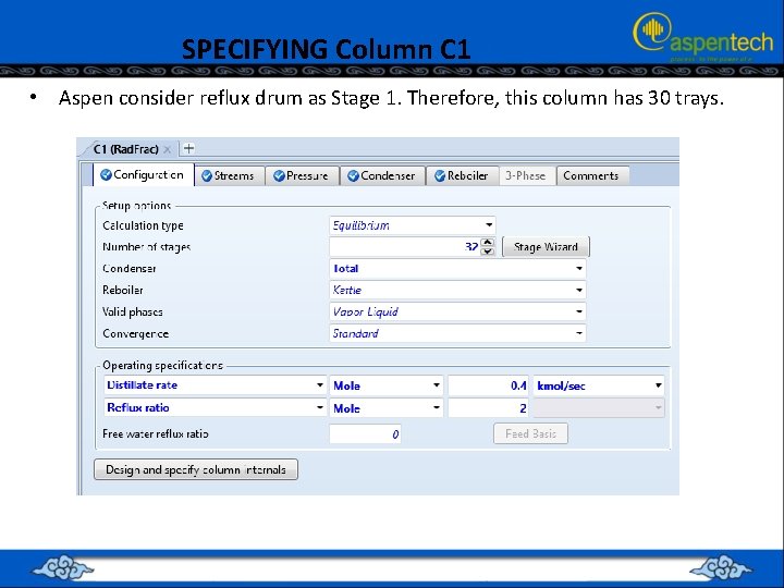
SPECIFYING Column C 1 • Aspen consider reflux drum as Stage 1. Therefore, this column has 30 trays.

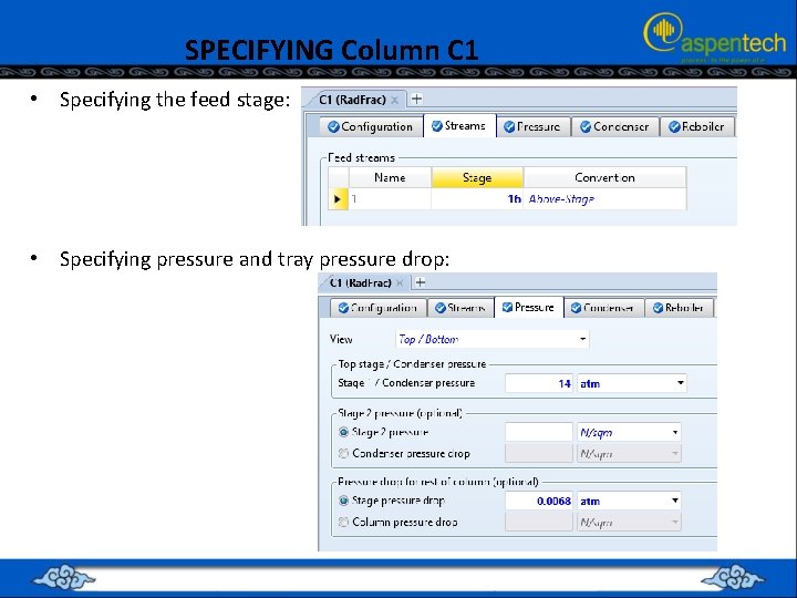
SPECIFYING Column C 1 • Specifying the feed stage: • Specifying pressure and tray pressure drop:

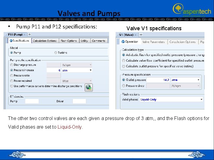
Valves and Pumps • Pump P 11 and P 12 specifications: Valve V 1 specifications The other two control valves are each given a pressure drop of 3 atm, , and the Flash options for Valid phases are set to Liquid-Only.

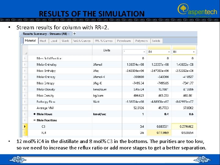
RESULTS OF THE SIMULATION • Stream results for column with RR=2. • 12 mol% i. C 4 in the distillate and 8 mol% C 3 in the bottoms. The purities are too low, so we need to increase the reflux ratio or add more stages to get a better separation.

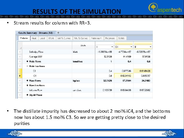
RESULTS OF THE SIMULATION • Stream results for column with RR=3. • The distillate impurity has decreased to about 2 mol% i. C 4, and the bottoms now has about 1. 5 mol% C 3. So we are getting pretty close to the desired purities

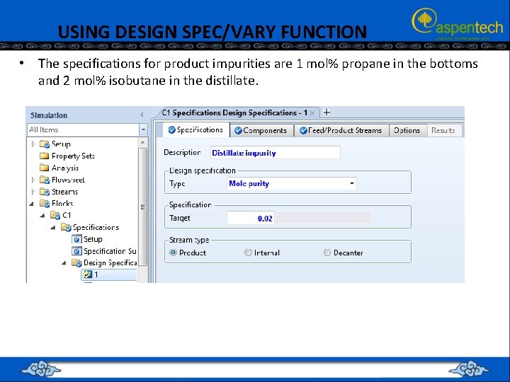
USING DESIGN SPEC/VARY FUNCTION • The specifications for product impurities are 1 mol% propane in the bottoms and 2 mol% isobutane in the distillate.

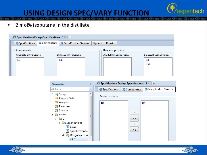
USING DESIGN SPEC/VARY FUNCTION • 2 mol% isobutane in the distillate.

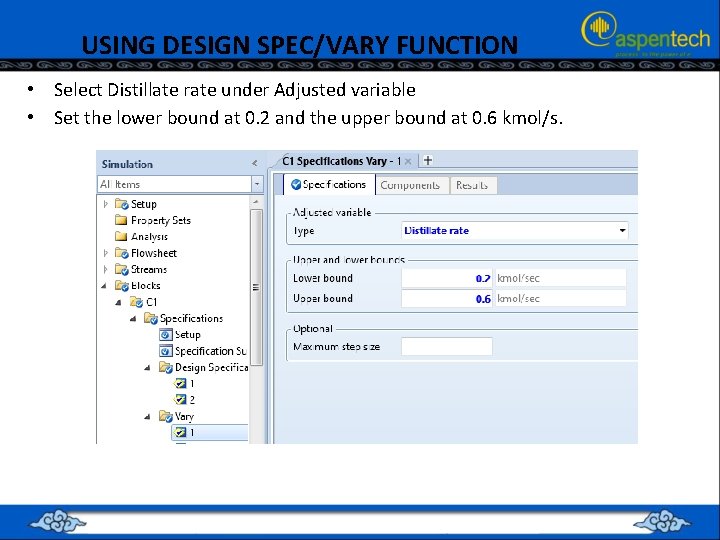
USING DESIGN SPEC/VARY FUNCTION • Select Distillate rate under Adjusted variable • Set the lower bound at 0. 2 and the upper bound at 0. 6 kmol/s.

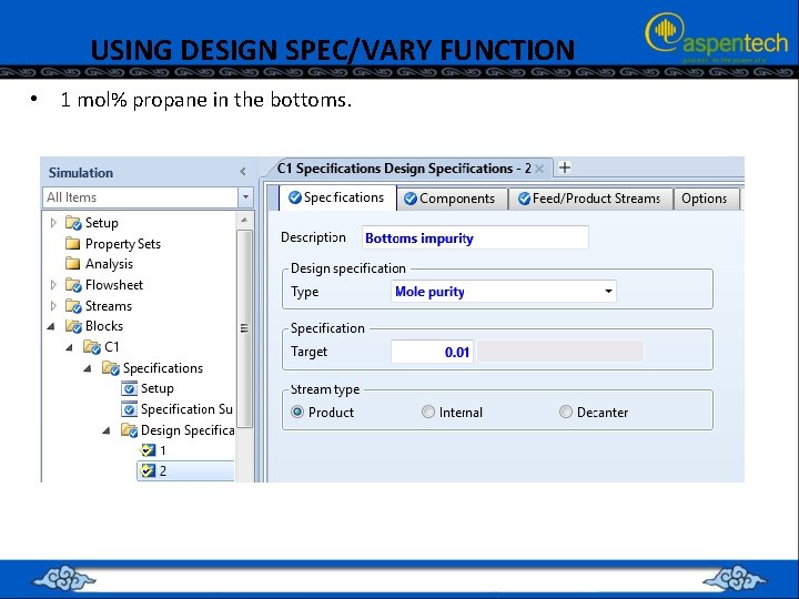
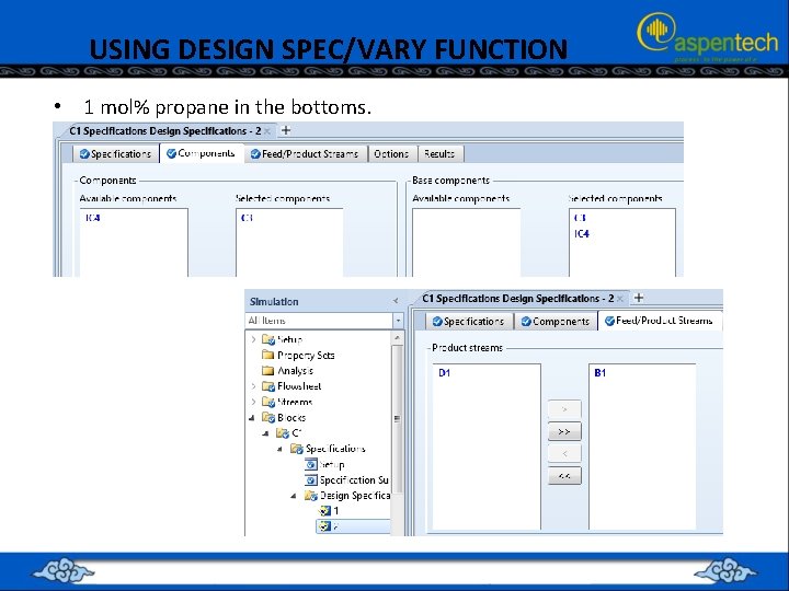
USING DESIGN SPEC/VARY FUNCTION • 1 mol% propane in the bottoms.

USING DESIGN SPEC/VARY FUNCTION • 1 mol% propane in the bottoms.

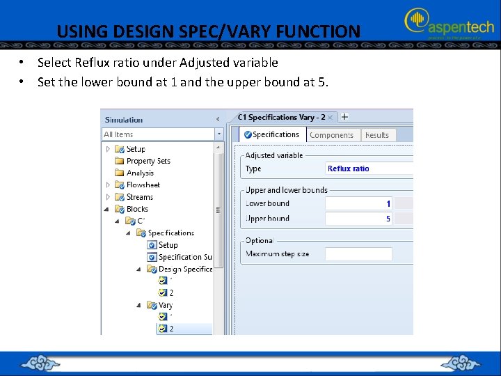
USING DESIGN SPEC/VARY FUNCTION • Select Reflux ratio under Adjusted variable • Set the lower bound at 1 and the upper bound at 5.

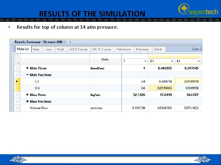
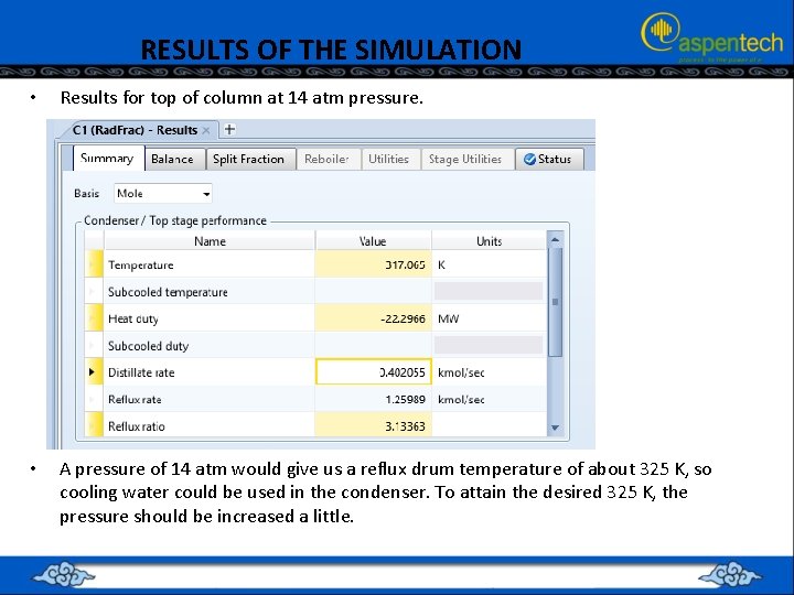
RESULTS OF THE SIMULATION • Results for top of column at 14 atm pressure.

RESULTS OF THE SIMULATION • Results for top of column at 14 atm pressure. • A pressure of 14 atm would give us a reflux drum temperature of about 325 K, so cooling water could be used in the condenser. To attain the desired 325 K, the pressure should be increased a little.

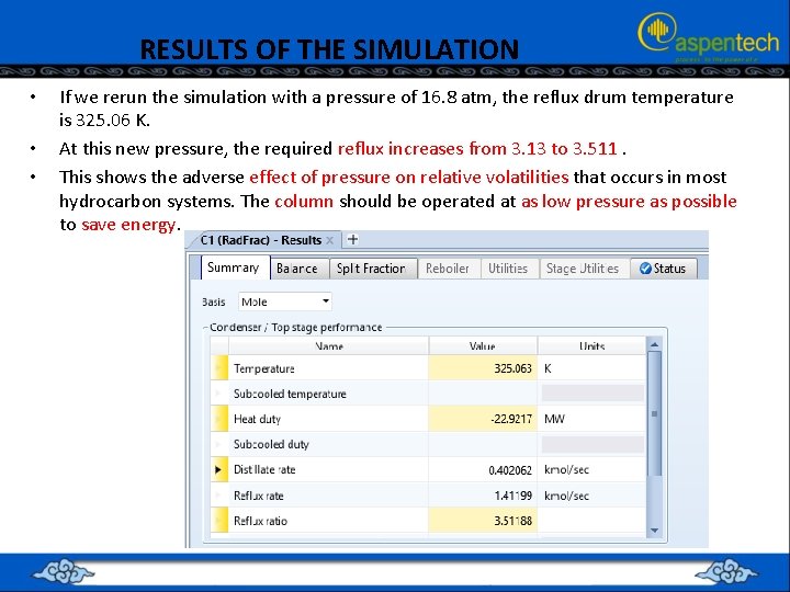
RESULTS OF THE SIMULATION • • • If we rerun the simulation with a pressure of 16. 8 atm, the reflux drum temperature is 325. 06 K. At this new pressure, the required reflux increases from 3. 13 to 3. 511. This shows the adverse effect of pressure on relative volatilities that occurs in most hydrocarbon systems. The column should be operated at as low pressure as possible to save energy.

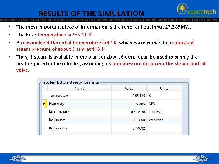
RESULTS OF THE SIMULATION • • The most important piece of information is the reboiler heat input 27. 385 MW. The base temperature is 366. 11 K. A reasonable differential temperature is 40 K, which corresponds to a saturated steam pressure of about 3 atm at 406 K. Thus, if steam is available in the plant at about 6 atm, it can be used to supply the heat required in the reboiler, assuming a 3 atm pressure drop over the steam control valve.

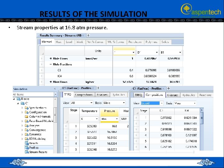
RESULTS OF THE SIMULATION • Stream properties at 16. 8 atm pressure.

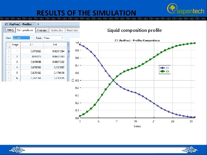
RESULTS OF THE SIMULATION Liquid composition profile

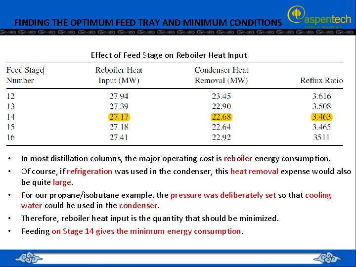
FINDING THE OPTIMUM FEED TRAY AND MINIMUM CONDITIONS Effect of Feed Stage on Reboiler Heat Input • • • In most distillation columns, the major operating cost is reboiler energy consumption. Of course, if refrigeration was used in the condenser, this heat removal expense would also be quite large. For our propane/isobutane example, the pressure was deliberately set so that cooling water could be used in the condenser. Therefore, reboiler heat input is the quantity that should be minimized. Feeding on Stage 14 gives the minimum energy consumption.

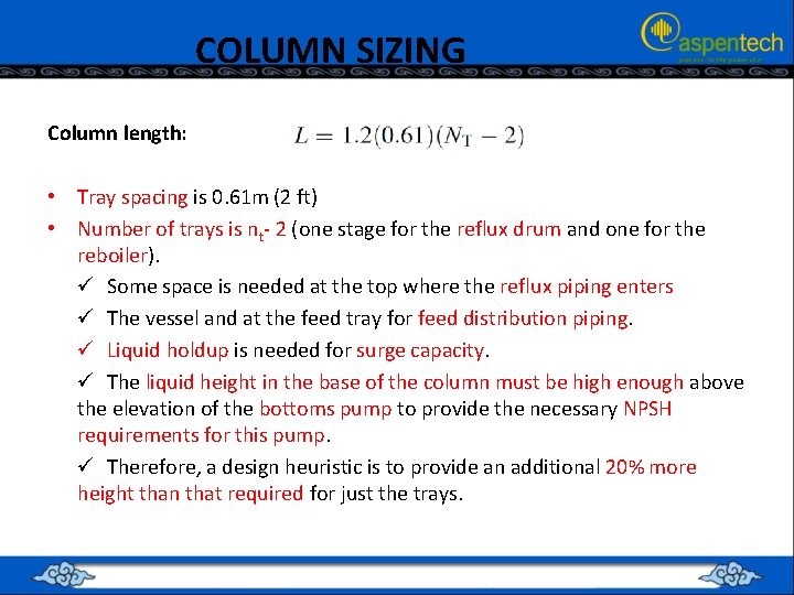
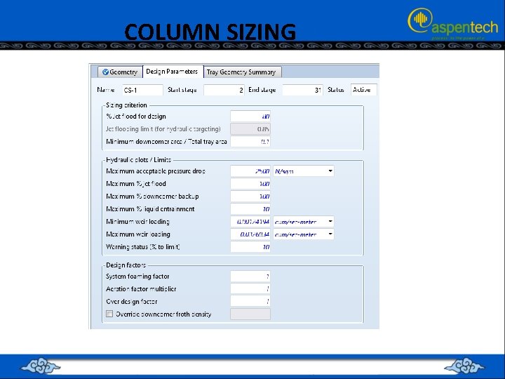
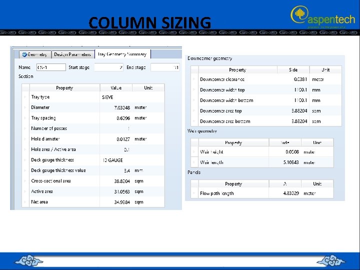
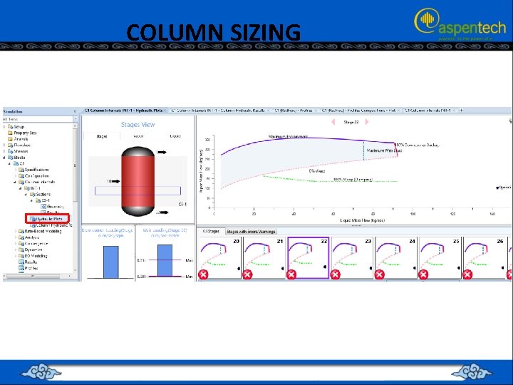
COLUMN SIZING Column length: • Tray spacing is 0. 61 m (2 ft) • Number of trays is nt- 2 (one stage for the reflux drum and one for the reboiler). ü Some space is needed at the top where the reflux piping enters ü The vessel and at the feed tray for feed distribution piping. ü Liquid holdup is needed for surge capacity. ü The liquid height in the base of the column must be high enough above the elevation of the bottoms pump to provide the necessary NPSH requirements for this pump. ü Therefore, a design heuristic is to provide an additional 20% more height than that required for just the trays.

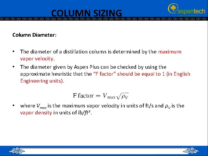
COLUMN SIZING Column Diameter: • The diameter of a distillation column is determined by the maximum vapor velocity. • The diameter given by Aspen Plus can be checked by using the approximate heuristic that the “F factor” should be equal to 1 (in English Engineering units). • where Vmax is the maximum vapor velocity in units of ft/s and ρV is the vapor density in units of lb/ft 3.

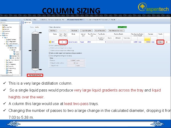
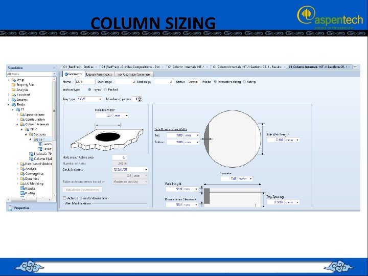
COLUMN SIZING ü This is a very large distillation column. ü So a single liquid pass would produce very large liquid gradients across the tray and liquid heights over the weir. ü A column this large would use at least two-pass trays. ü Changing the number of passes to two a large change in the calculated diameter, dropping it from 7. 03 to 5. 38 m.

COLUMN SIZING

COLUMN SIZING

COLUMN SIZING

COLUMN SIZING

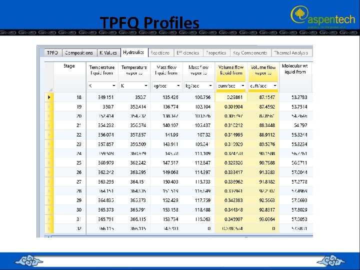
TPFQ Profiles

CONCEPTUAL DESIGN Using Aspen Plus® V 9. 0

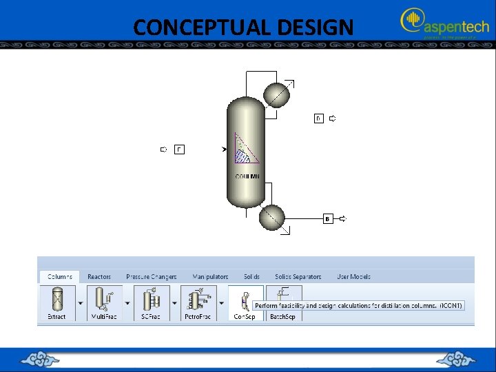
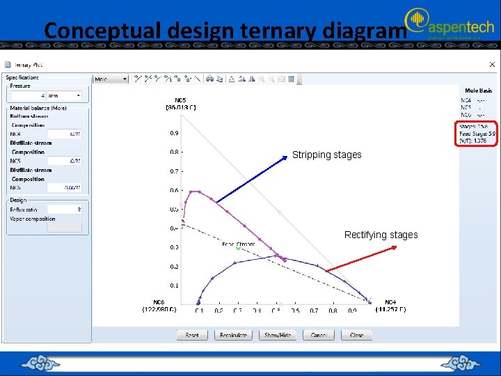
CONCEPTUAL DESIGN • The steady-state simulation of distillation columns in Aspen Plus discussed in previous sections took a “rating” approach to the problem. • Specific values for the total number of trays and the feed-tray location were selected, and the required reflux ratio and reboiler duty were determined for this specific configuration, subjected to attaining the desired product specifications. • Then, economics must be used to find what the optimum tray configuration is. • Aspen Plus provides feature called Conceptual Design that offers another approach to the problem (a “design” approach). • In this method, the product specifications are set at both ends of the column, as is a reflux ratio. Then, the program performs tray-to-tray calculations, both up and down the column, creating composition profiles for both the rectifying and stripping sections. If these two composition profile intersect, the reflux ratio selected is above the minimum, and the number of trays in both sections is now known. • The method is applicable to ternary systems with a single feed stream.

CONCEPTUAL DESIGN

CONCEPTUAL DESIGN

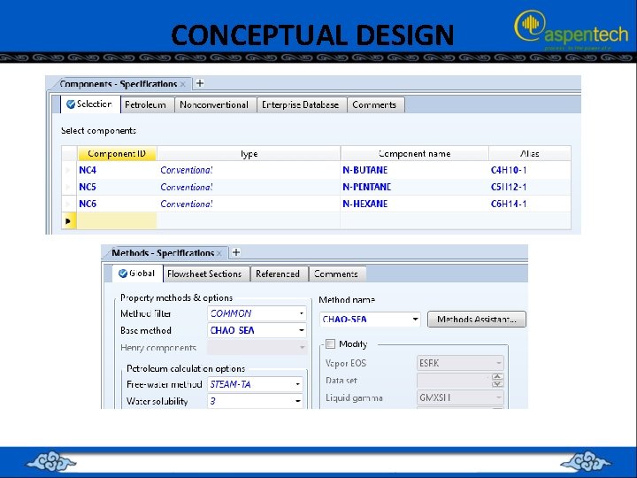
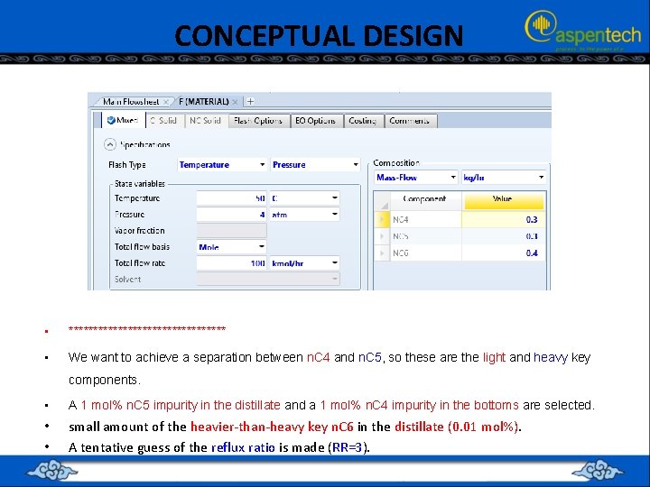
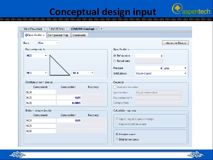
CONCEPTUAL DESIGN • **************** • We want to achieve a separation between n. C 4 and n. C 5, so these are the light and heavy key components. • A 1 mol% n. C 5 impurity in the distillate and a 1 mol% n. C 4 impurity in the bottoms are selected. • • small amount of the heavier-than-heavy key n. C 6 in the distillate (0. 01 mol%). A tentative guess of the reflux ratio is made (RR=3).

Conceptual design input

Conceptual design ternary diagram Stripping stages Rectifying stages

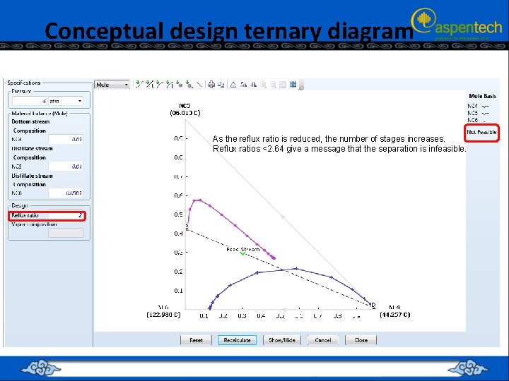
Conceptual design ternary diagram As the reflux ratio is reduced, the number of stages increases. Reflux ratios <2. 64 give a message that the separation is infeasible.

DISTILLATION ECONOMIC OPTIMIZATION Using Aspen Plus® V 9. 0

DISTILLATION ECONOMIC OPTIMIZATION • we need to find the optimum number of total stages. • There are some simple approaches, and there are more rigorous approaches. • The simple methods use heuristics such as setting the total number of trays equal to twice the minimum. • The rigorous methods look at how the capital and energy costs change with the number of trays and find the configuration of stages (total and feed stage) that gives the minimum total annual cost (TAC).

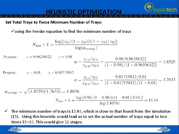
HEURISTIC OPTIMIZATION Set Total Trays to Twice Minimum Number of Trays: üusing the Fenske equation to find the minimum number of trays ü The minimum number of trays is 13. 43, which is close to that found from the simulation (15). Using this heuristic would lead us to set the actual number of trays equal to two times 15=30. This would give 32 stages.

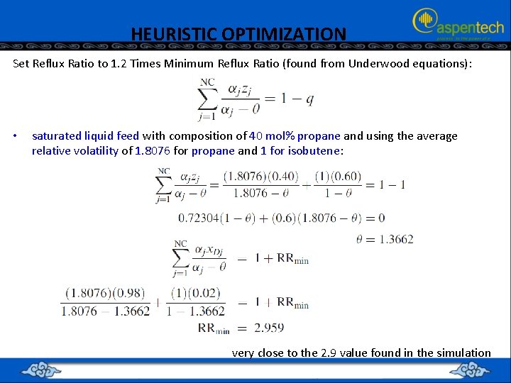
HEURISTIC OPTIMIZATION Set Reflux Ratio to 1. 2 Times Minimum Reflux Ratio (found from Underwood equations): • saturated liquid feed with composition of 40 mol% propane and using the average relative volatility of 1. 8076 for propane and 1 for isobutene: very close to the 2. 9 value found in the simulation

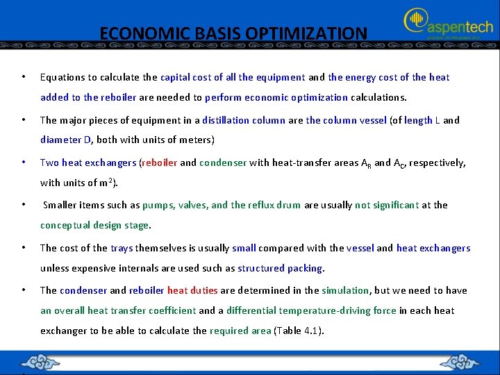
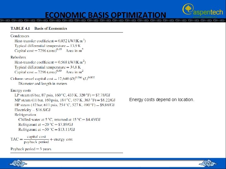
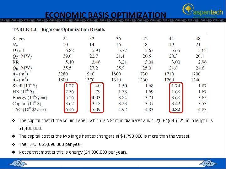
ECONOMIC BASIS OPTIMIZATION • Equations to calculate the capital cost of all the equipment and the energy cost of the heat added to the reboiler are needed to perform economic optimization calculations. • The major pieces of equipment in a distillation column are the column vessel (of length L and diameter D, both with units of meters) • Two heat exchangers (reboiler and condenser with heat-transfer areas AR and AC, respectively, with units of m 2). • Smaller items such as pumps, valves, and the reflux drum are usually not significant at the conceptual design stage. • The cost of the trays themselves is usually small compared with the vessel and heat exchangers unless expensive internals are used such as structured packing. • The condenser and reboiler heat duties are determined in the simulation, but we need to have an overall heat transfer coefficient and a differential temperature-driving force in each heat exchanger to be able to calculate the required area (Table 4. 1).

ECONOMIC BASIS OPTIMIZATION Energy costs depend on location.

ECONOMIC BASIS OPTIMIZATION

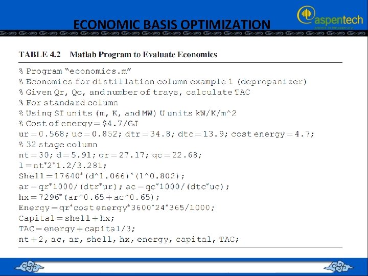
ECONOMIC BASIS OPTIMIZATION v The capital cost of the column shell, which is 5. 91 m in diameter and 1. 2(0. 61)(30)=22 m in length, is $1, 400, 000. v The capital cost of the two large heat exchangers at $1, 790, 000 is more than the vessel. v The TAC is $5, 090, 000 per year. v Notice that most of this is energy ($4, 030, 000 per year).

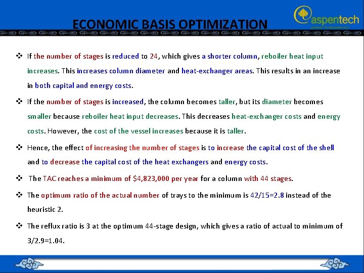
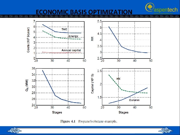
ECONOMIC BASIS OPTIMIZATION v If the number of stages is reduced to 24, which gives a shorter column, reboiler heat input increases. This increases column diameter and heat-exchanger areas. This results in an increase in both capital and energy costs. v If the number of stages is increased, the column becomes taller, but its diameter becomes smaller because reboiler heat input decreases. This decreases heat-exchanger costs and energy costs. However, the cost of the vessel increases because it is taller. v Hence, the effect of increasing the number of stages is to increase the capital cost of the shell and to decrease the capital cost of the heat exchangers and energy costs. v The TAC reaches a minimum of $4, 823, 000 per year for a column with 44 stages. v The optimum ratio of the actual number of trays to the minimum is 42/15=2. 8 instead of the heuristic 2. v The reflux ratio is 3 at the optimum 44 -stage design, which gives a ratio of actual to minimum of 3/2. 9=1. 04.

ECONOMIC BASIS OPTIMIZATION

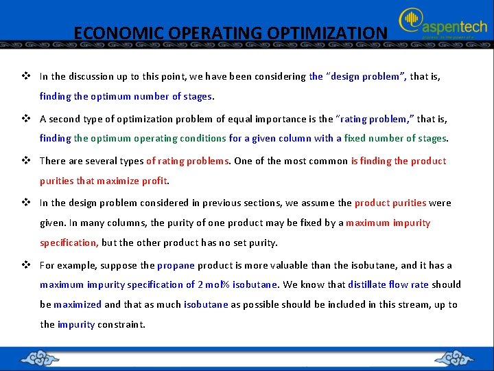
ECONOMIC OPERATING OPTIMIZATION v In the discussion up to this point, we have been considering the “design problem”, that is, finding the optimum number of stages. v A second type of optimization problem of equal importance is the “rating problem, ” that is, finding the optimum operating conditions for a given column with a fixed number of stages. v There are several types of rating problems. One of the most common is finding the product purities that maximize profit. v In the design problem considered in previous sections, we assume the product purities were given. In many columns, the purity of one product may be fixed by a maximum impurity specification, but the other product has no set purity. v For example, suppose the propane product is more valuable than the isobutane, and it has a maximum impurity specification of 2 mol% isobutane. We know that distillate flow rate should be maximized and that as much isobutane as possible should be included in this stream, up to the impurity constraint.

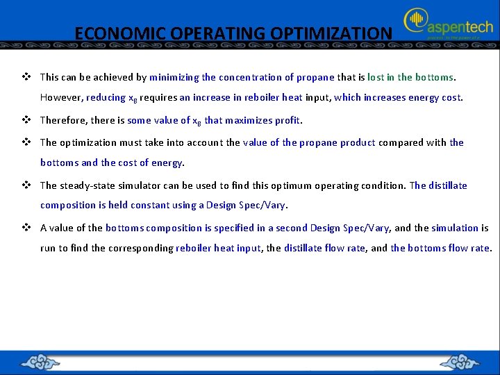
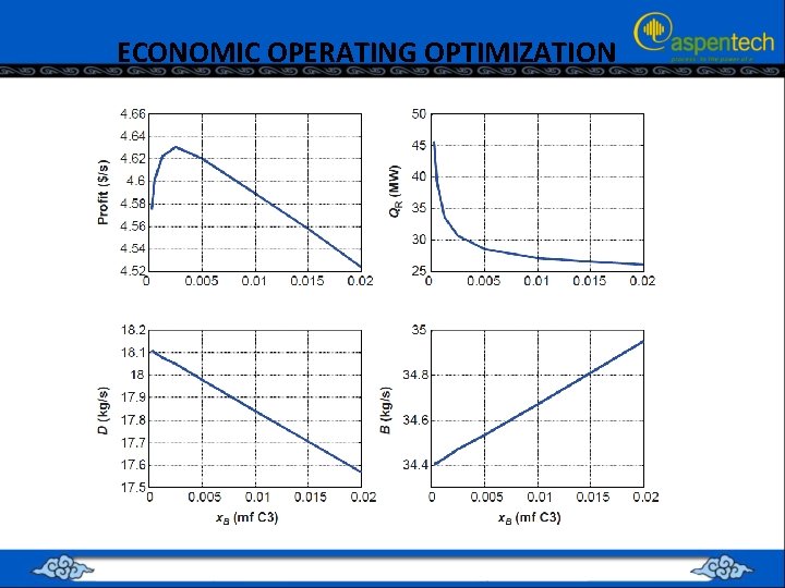
ECONOMIC OPERATING OPTIMIZATION v This can be achieved by minimizing the concentration of propane that is lost in the bottoms. However, reducing x. B requires an increase in reboiler heat input, which increases energy cost. v Therefore, there is some value of x. B that maximizes profit. v The optimization must take into account the value of the propane product compared with the bottoms and the cost of energy. v The steady-state simulator can be used to find this optimum operating condition. The distillate composition is held constant using a Design Spec/Vary. v A value of the bottoms composition is specified in a second Design Spec/Vary, and the simulation is run to find the corresponding reboiler heat input, the distillate flow rate, and the bottoms flow rate.

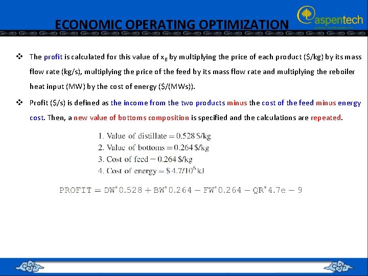
ECONOMIC OPERATING OPTIMIZATION v The profit is calculated for this value of x. B by multiplying the price of each product ($/kg) by its mass flow rate (kg/s), multiplying the price of the feed by its mass flow rate and multiplying the reboiler heat input (MW) by the cost of energy ($/(MWs)). v Profit ($/s) is defined as the income from the two products minus the cost of the feed minus energy cost. Then, a new value of bottoms composition is specified and the calculations are repeated.

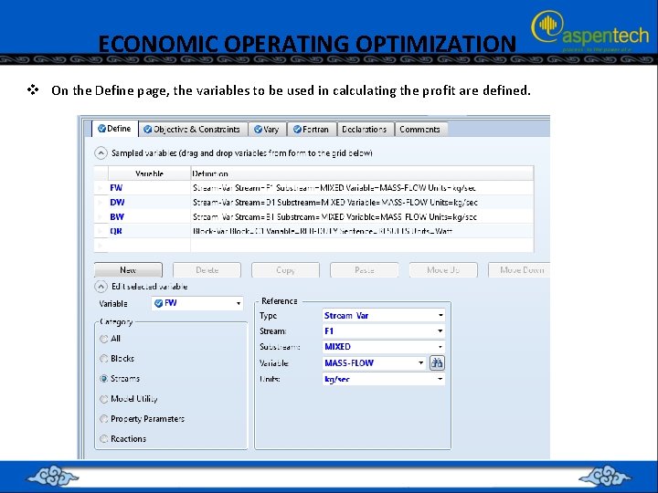
ECONOMIC OPERATING OPTIMIZATION v On the Define page, the variables to be used in calculating the profit are defined.

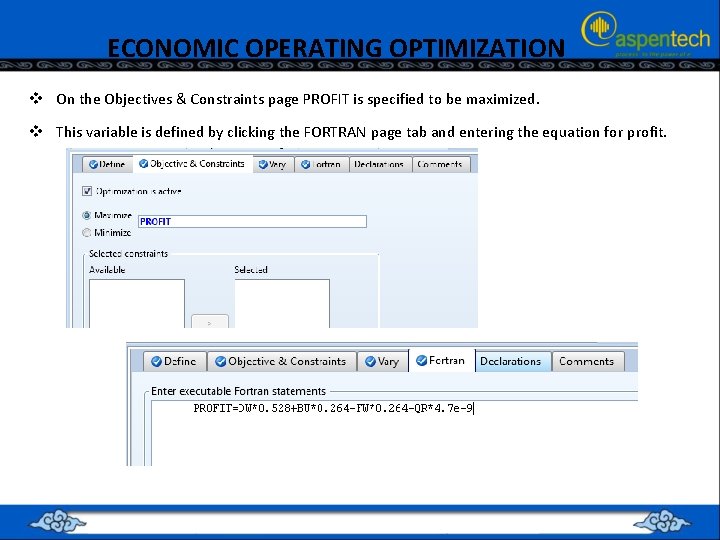
ECONOMIC OPERATING OPTIMIZATION v On the Objectives & Constraints page PROFIT is specified to be maximized. v This variable is defined by clicking the FORTRAN page tab and entering the equation for profit.

ECONOMIC OPERATING OPTIMIZATION v On the Objectives & Constraints page PROFIT is specified to be maximized. v This variable is defined by clicking the FORTRAN page tab and entering the equation for profit.

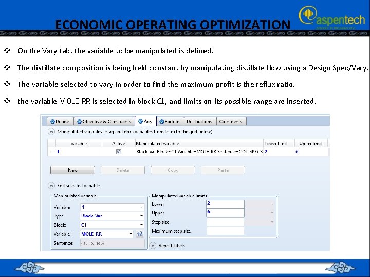
ECONOMIC OPERATING OPTIMIZATION v On the Vary tab, the variable to be manipulated is defined. v The distillate composition is being held constant by manipulating distillate flow using a Design Spec/Vary. v The variable selected to vary in order to find the maximum profit is the reflux ratio. v the variable MOLE-RR is selected in block C 1, and limits on its possible range are inserted.

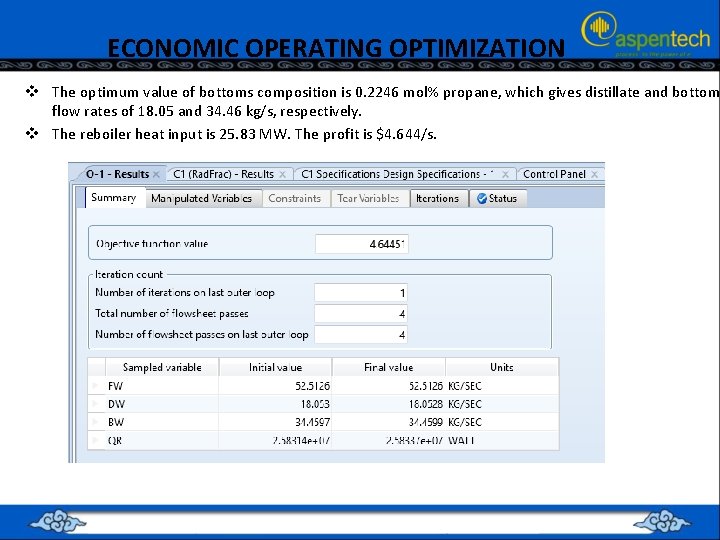
ECONOMIC OPERATING OPTIMIZATION v The optimum value of bottoms composition is 0. 2246 mol% propane, which gives distillate and bottom flow rates of 18. 05 and 34. 46 kg/s, respectively. v The reboiler heat input is 25. 83 MW. The profit is $4. 644/s.

ECONOMIC OPERATING OPTIMIZATION

ETHANOL DEHYDRATION