CHEMICAL ENGINEERING THERMODYANAMICSII EVALUATION OF ACTIVITY COEFFICENT Prepared

CHEMICAL ENGINEERING THERMODYANAMICS-II EVALUATION OF ACTIVITY COEFFICENT Prepared By Hitesh N. Panchal Assistant Professor D. D. University Nadiad. 1

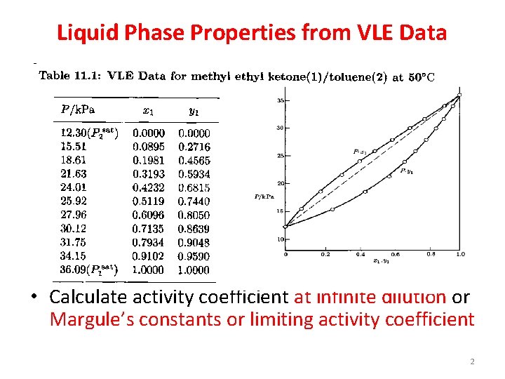
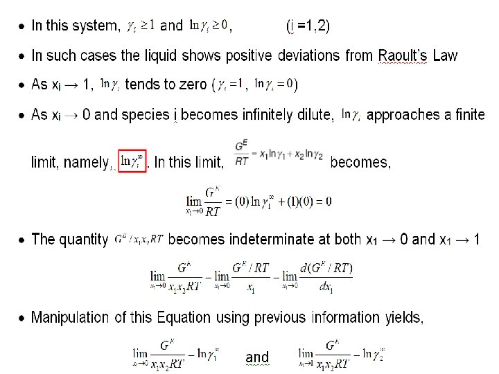
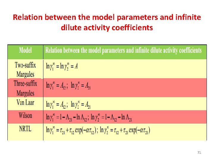
Liquid Phase Properties from VLE Data • Calculate activity coefficient at infinite dilution or Margule’s constants or limiting activity coefficient 2

Infinite dilution • It is the particular behavior of a two substances mixture when the concentration of one component approaches the limit of zero and the other approaches 1(second component being the solvent). • Behavior when the mixture is sufficiently dilute that solute-solute interactions are negligeble. 3

Importance and use of infinite dilution activity coefficient data • Most difficult and costly stage of a separation process is the removal of the last traces of impurity. • Greatest departure from ideality occurs in the very dilute regions • Synthesis, design and optimization of separation processes • Predicting the existence of an azeotropes

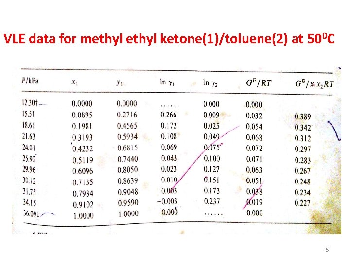
VLE data for methyl ketone(1)/toluene(2) at 500 C 5

6

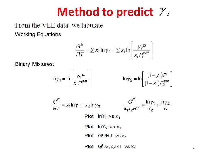
Method to predict 7

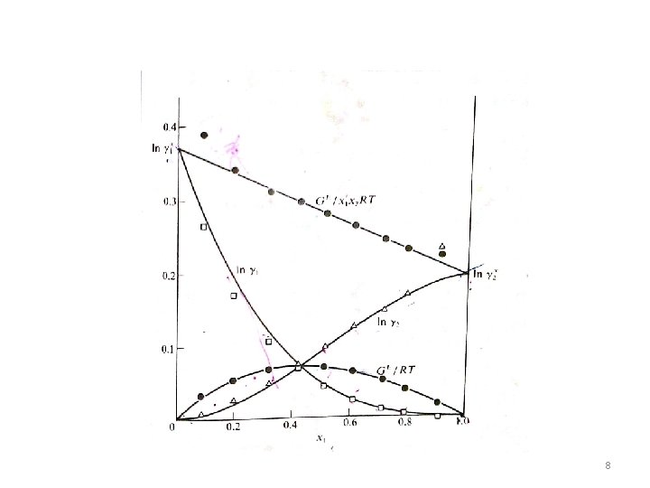
8

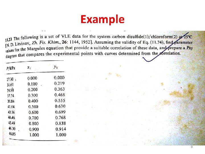
Example 9

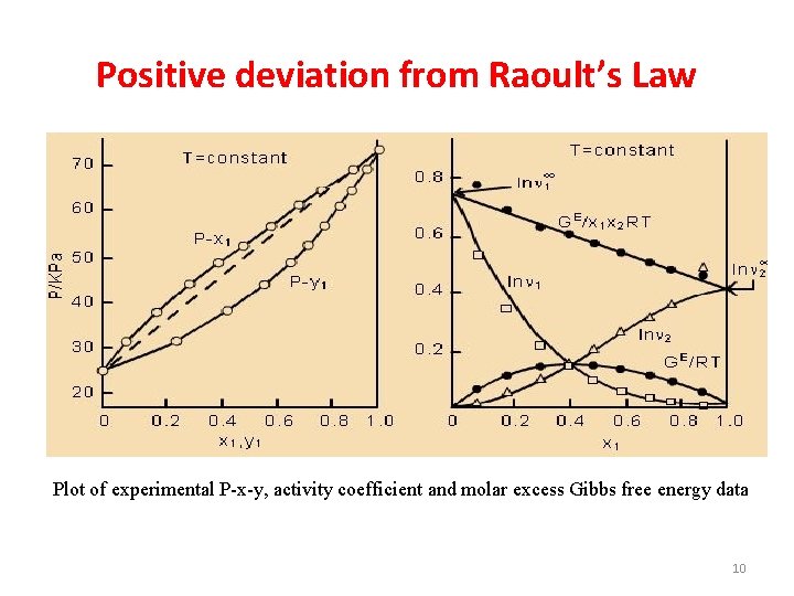
Positive deviation from Raoult’s Law Plot of experimental P-x-y, activity coefficient and molar excess Gibbs free energy data 10

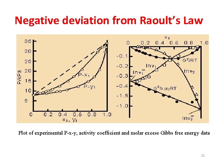
Negative deviation from Raoult’s Law Plot of experimental P-x-y, activity coefficient and molar excess Gibbs free energy data 11

Azeotropes • Importance of boiling point diagram(T-x-y diagram) & P-x -y diagram. • An Azeotrope is a mixture of two or more liquids in such a way that its components cannot be altered by simple distillation. • This happens because, when an azeotrope is boiled, the vapor has the same proportions of constituents as the unboiled mixture. • Because their composition is unchanged by distillation, azeotropes are also called constant boiling mixtures. 12

Azeotropes • In some real systems, the temperature / composition curve is far from ideal. • A maximum or minimum in the curve is possible; this is an azeotrope. • At the azeotrope, the liquid and vapor have the same composition. • Word azeotrope is derived from the Greek words, overall meaning, "no change on boiling". 13

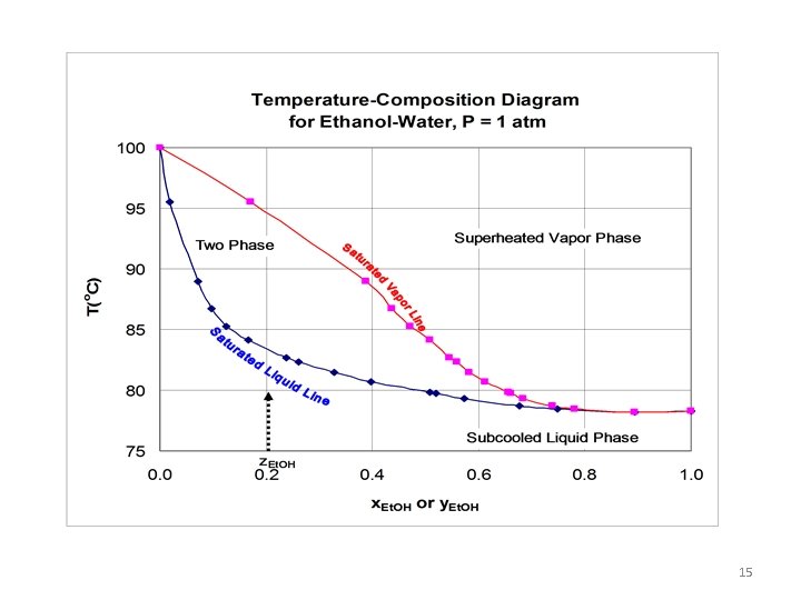
Ethanol-water system • A example of a positive azeotrope is 89. 44% ethanol and 11. 56% water (by weight). • Ethanol boils at 78. 4 °C, water boils at 100 °C, but the azeotrope boils at 78. 2 °C, which is lower than either of its constituents. • 78. 2 °C is the minimum temperature at which any ethanol/water solution can boil at atmospheric pressure. 14

15

• This limit is 0. 8943 mole fraction of ethanol for an ethanol-water mixture at P = 1 atm. • To separate a mixture containing 0. 9 ethanol liquid mole fraction at 1 atm • Azeotropes are dependent upon pressures and one way to avoid this problem is to vary the pressure. • For example, under a vacuum (P = 70 mm. Hg), no azeotrope exists for the ethanol-water mixture. This is one reason that vacuum distillation is often done for many separations. • Azetropes are often also component dependent. • For example, the addition of a 3 rd component to a binary system, may change or “break” the azeotrope.

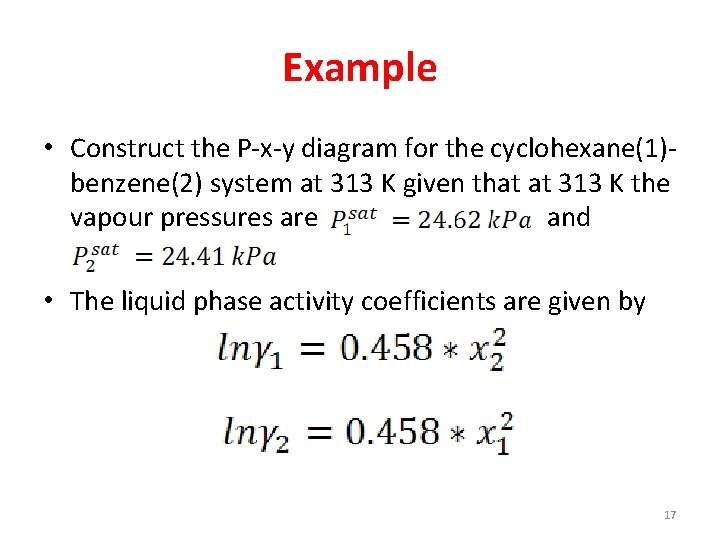
Example • Construct the P-x-y diagram for the cyclohexane(1)benzene(2) system at 313 K given that at 313 K the vapour pressures are and • The liquid phase activity coefficients are given by 17

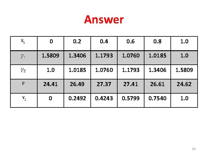
Answer 0 0. 2 0. 4 0. 6 0. 8 1. 0 1. 5809 1. 3406 1. 1793 1. 0760 1. 0185 1. 0760 1. 1793 1. 3406 1. 5809 P 24. 41 26. 49 27. 37 27. 41 26. 61 24. 62 Y 1 0 0. 2492 0. 4243 0. 5799 0. 7540 1. 0 X 1 18

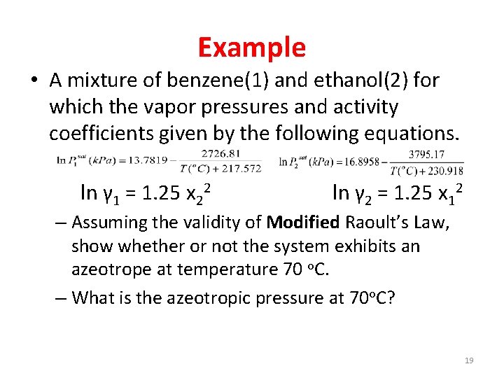
Example • A mixture of benzene(1) and ethanol(2) for which the vapor pressures and activity coefficients given by the following equations. ln γ 1 = 1. 25 x 22 ln γ 2 = 1. 25 x 12 – Assuming the validity of Modified Raoult’s Law, show whether or not the system exhibits an azeotrope at temperature 70 o. C. – What is the azeotropic pressure at 70 o. C? 19

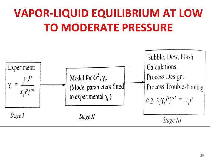
VAPOR-LIQUID EQUILIBRIUM AT LOW TO MODERATE PRESSURE 20

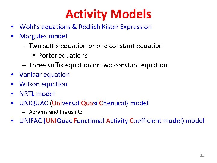
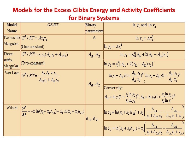
Activity Models • Wohl’s equations & Redlich Kister Expression • Margules model – Two suffix equation or one constant equation • Porter equations – Three suffix equation or two constant equation • Vanlaar equation • Wilson equation • NRTL model • UNIQUAC (Universal Quasi Chemical) model – Abrams and Prausnitz • UNIFAC (UNIQuac Functional Activity Coefficient model) model 21

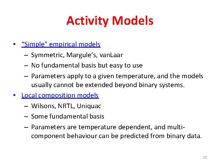
Activity Models • “Simple” empirical models – Symmetric, Margule’s, van. Laar – No fundamental basis but easy to use – Parameters apply to a given temperature, and the models usually cannot be extended beyond binary systems. • Local composition models – Wilsons, NRTL, Uniquac – Some fundamental basis – Parameters are temperature dependent, and multicomponent behaviour can be predicted from binary data. 22

VAPOR-LIQUID EQUILIBRIUM AT LOW PRESSURE • Various activity coefficient models commonly used for VLE calculations. • Divided into two major groups depending upon their applicability to various types of solutions: 1. Margules/Van Laar models • Homogeneous Mixture models 2. Wilson/NRTL (Non-Random Two Liquid)/UNIQUAC (Universal Quasi Chemical) Models • Local Composition models

• Non-ideal behavior of liquid solutions derives from two sources: – difference in molecular size/shape of constituent – difference between the molecular interaction energies. • Type 1 models generally apply to systems in which the inter-species and molecular interaction energies differ from each other. • Type 2 models are principally useful for describing systems where the constituent molecular species differ on account of both size/shape as well molecular interaction energies. 24

Models for Excess Gibbs free energy 25

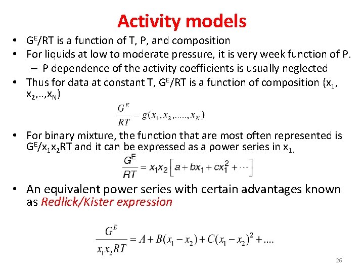
Activity models • GE/RT is a function of T, P, and composition • For liquids at low to moderate pressure, it is very week function of P. – P dependence of the activity coefficients is usually neglected • Thus for data at constant T, GE/RT is a function of composition (x 1, x 2, . . , x. N) • For binary mixture, the function that are most often represented is GE/x 1 x 2 RT and it can be expressed as a power series in x 1. • An equivalent power series with certain advantages known as Redlick/Kister expression 26

Derivation of Margules Equations 27

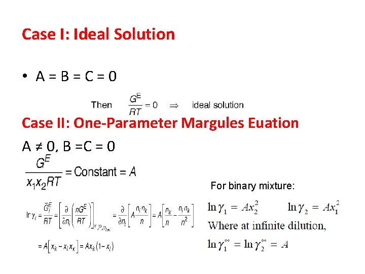
Margules equation Max Margules introduced in 1895 a simple thermodynamic model for the excess Gibbs free energy of a liquid mixture. He had introduced the concept of the activity coefficient, the model could be used to derive an expression for the activity coefficients of a compound i in a liquid. 28

Case I: Ideal Solution • A = B = C = 0 Case II: One-Parameter Margules Euation A ≠ 0, B =C = 0 For binary mixture:

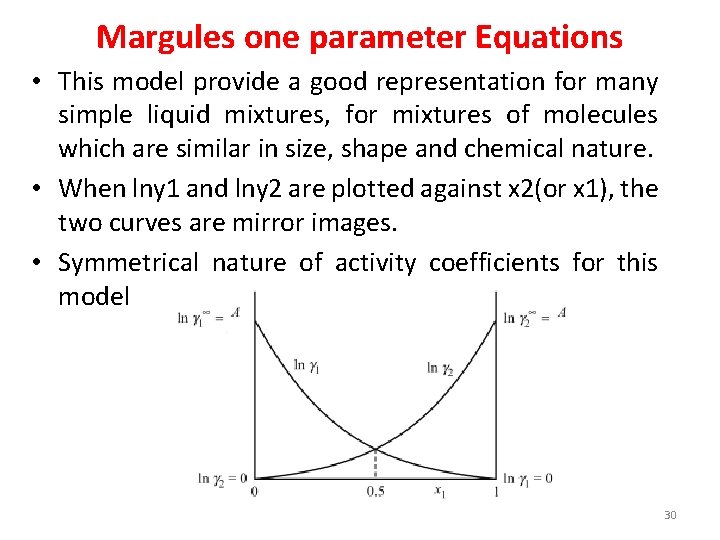
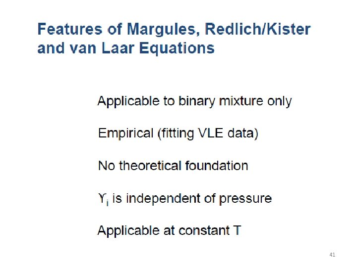
Margules one parameter Equations • This model provide a good representation for many simple liquid mixtures, for mixtures of molecules which are similar in size, shape and chemical nature. • When lny 1 and lny 2 are plotted against x 2(or x 1), the two curves are mirror images. • Symmetrical nature of activity coefficients for this model 30

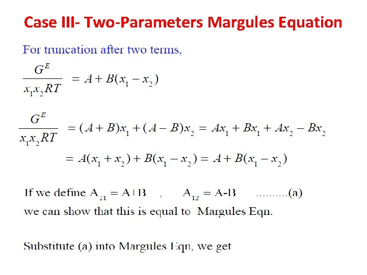
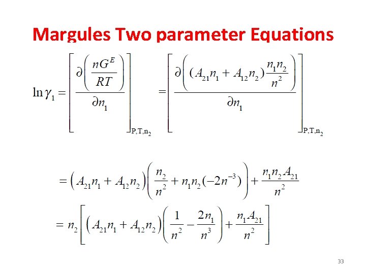
Case III- Two-Parameters Margules Equation

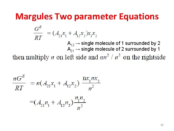
Margules Two parameter Equations A 12 → single molecule of 1 surrounded by 2 A 21 → single molecule of 2 surrounded by 1 32

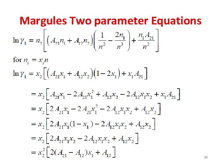
Margules Two parameter Equations 33

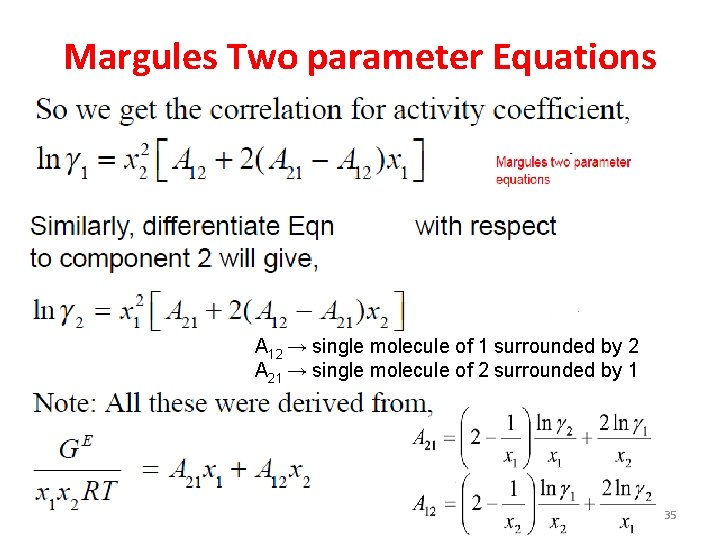
Margules Two parameter Equations 34

Margules Two parameter Equations A 12 → single molecule of 1 surrounded by 2 A 21 → single molecule of 2 surrounded by 1 35

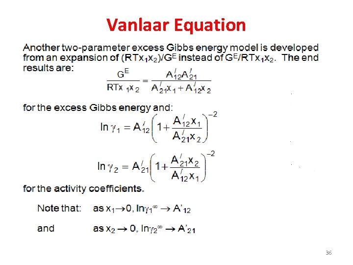
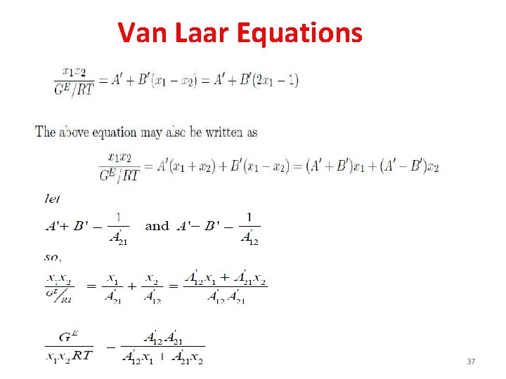
Vanlaar Equation 36

Van Laar Equations 37

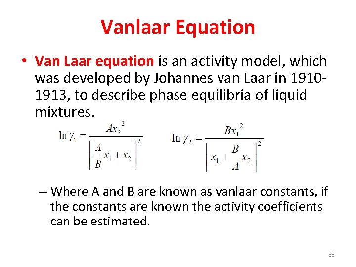
Vanlaar Equation • Van Laar equation is an activity model, which was developed by Johannes van Laar in 19101913, to describe phase equilibria of liquid mixtures. – Where A and B are known as vanlaar constants, if the constants are known the activity coefficients can be estimated. 38

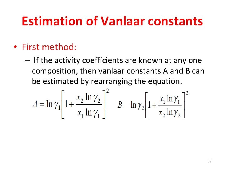
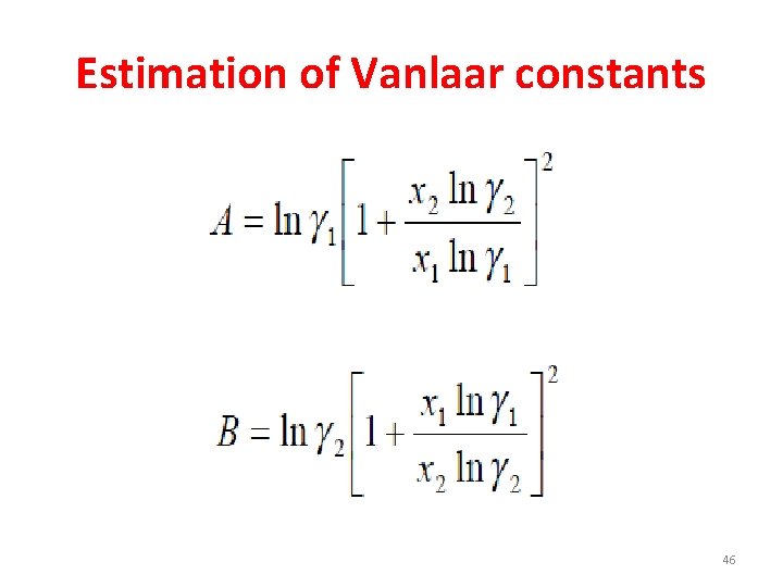
Estimation of Vanlaar constants • First method: – If the activity coefficients are known at any one composition, then vanlaar constants A and B can be estimated by rearranging the equation. 39

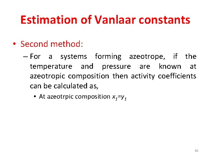
Estimation of Vanlaar constants • Second method: – For a systems forming azeotrope, if the temperature and pressure are known at azeotropic composition then activity coefficients can be calculated as, • At azeotrpic composition x 1=y 1 40

41

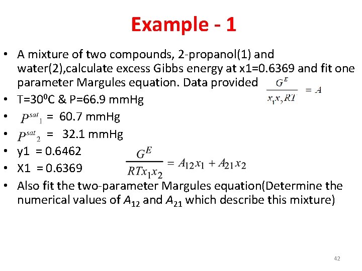
Example - 1 • A mixture of two compounds, 2 -propanol(1) and water(2), calculate excess Gibbs energy at x 1=0. 6369 and fit one parameter Margules equation. Data provided • T=300 C & P=66. 9 mm. Hg • = 60. 7 mm. Hg • = 32. 1 mm. Hg • y 1 = 0. 6462 • X 1 = 0. 6369 • Also fit the two-parameter Margules equation(Determine the numerical values of A 12 and A 21 which describe this mixture) 42

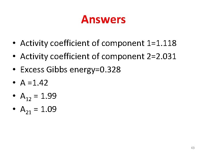
Answers • • • Activity coefficient of component 1=1. 118 Activity coefficient of component 2=2. 031 Excess Gibbs energy=0. 328 A =1. 42 A 12 = 1. 99 A 21 = 1. 09 43

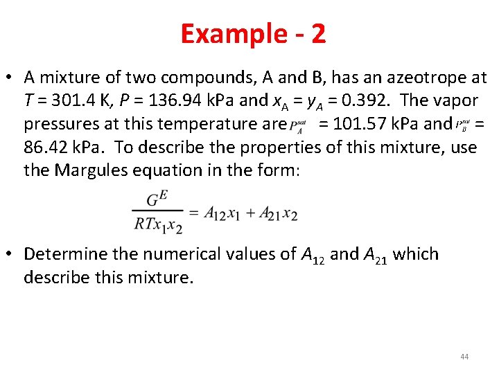
Example - 2 • A mixture of two compounds, A and B, has an azeotrope at T = 301. 4 K, P = 136. 94 k. Pa and x. A = y. A = 0. 392. The vapor pressures at this temperature are = 101. 57 k. Pa and = 86. 42 k. Pa. To describe the properties of this mixture, use the Margules equation in the form: • Determine the numerical values of A 12 and A 21 which describe this mixture. 44

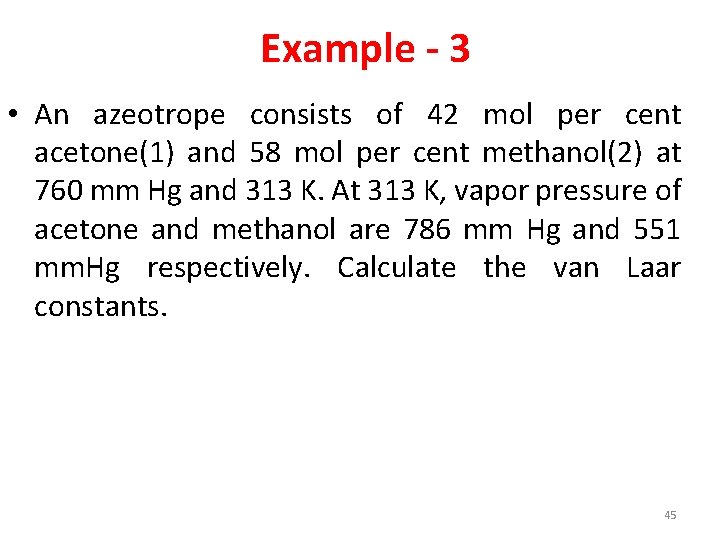
Example - 3 • An azeotrope consists of 42 mol per cent acetone(1) and 58 mol per cent methanol(2) at 760 mm Hg and 313 K. At 313 K, vapor pressure of acetone and methanol are 786 mm Hg and 551 mm. Hg respectively. Calculate the van Laar constants. 45

Estimation of Vanlaar constants 46

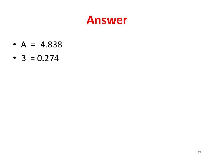
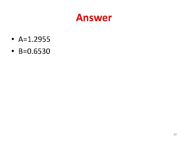
Answer • A = -4. 838 • B = 0. 274 47

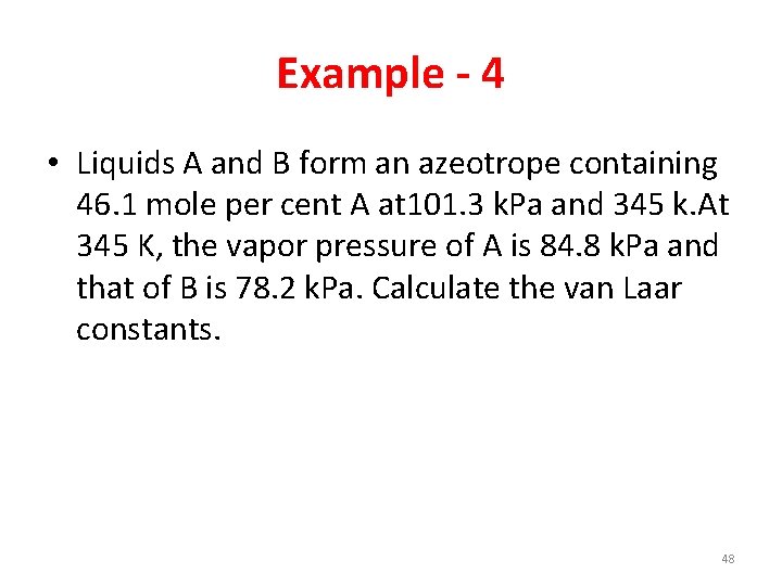
Example - 4 • Liquids A and B form an azeotrope containing 46. 1 mole per cent A at 101. 3 k. Pa and 345 k. At 345 K, the vapor pressure of A is 84. 8 k. Pa and that of B is 78. 2 k. Pa. Calculate the van Laar constants. 48

Answer • A=1. 2955 • B=0. 6530 49

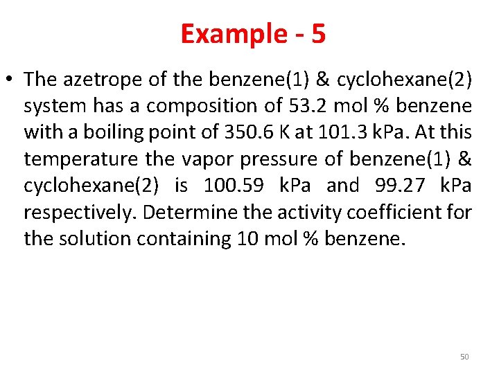
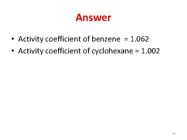
Example - 5 • The azetrope of the benzene(1) & cyclohexane(2) system has a composition of 53. 2 mol % benzene with a boiling point of 350. 6 K at 101. 3 k. Pa. At this temperature the vapor pressure of benzene(1) & cyclohexane(2) is 100. 59 k. Pa and 99. 27 k. Pa respectively. Determine the activity coefficient for the solution containing 10 mol % benzene. 50

Answer • Activity coefficient of benzene = 1. 062 • Activity coefficient of cyclohexane = 1. 002 51

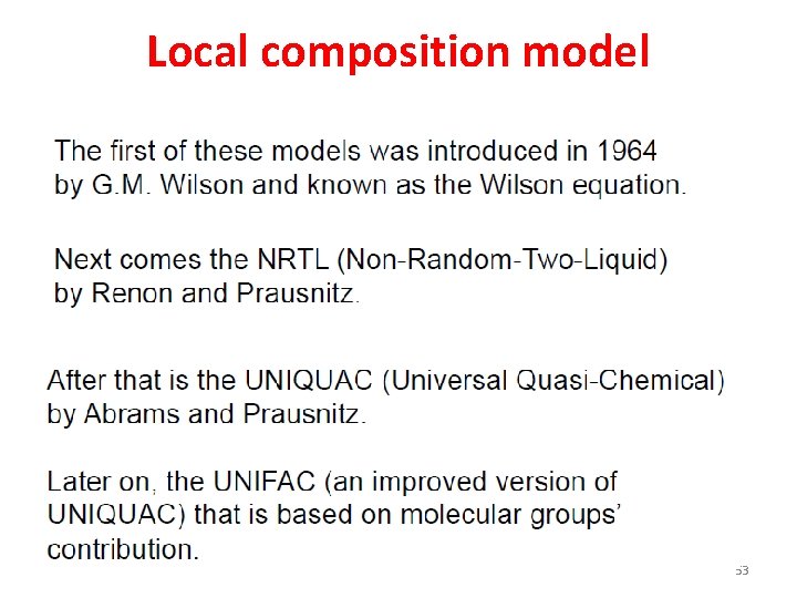
Local composition models • Concept of LCMs is based on the hypothesis of that the local concentration around a molecule is different from the bulk concentration. • Local composition is incorporated to model to account for the nonrandom molecular orientations resulting from differences in molecular size and intermolecular forces. – This difference is due to a difference between the interaction energy of the central molecule with the molecules of its own kind and that with the molecules of the other kind. – Energy difference also introduces a non-randomness at the local molecular level. 52

Local composition model 53

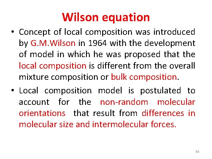
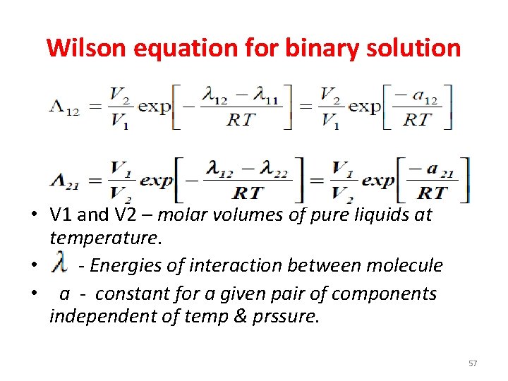
Wilson equation • Concept of local composition was introduced by G. M. Wilson in 1964 with the development of model in which he was proposed that the local composition is different from the overall mixture composition or bulk composition. • Local composition model is postulated to account for the non-random molecular orientations that result from differences in molecular size and intermolecular forces. 54

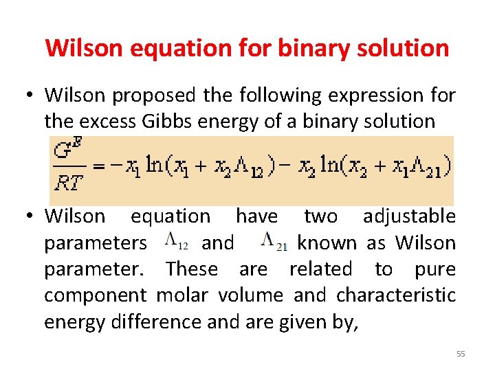
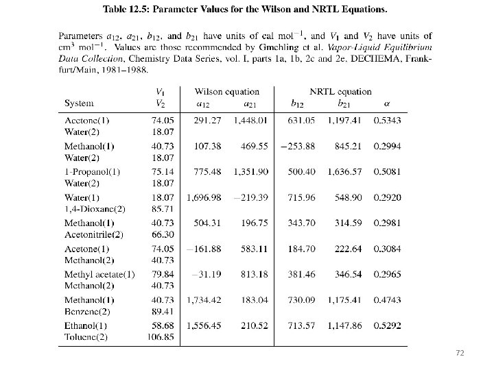
Wilson equation for binary solution • Wilson proposed the following expression for the excess Gibbs energy of a binary solution • Wilson equation have two adjustable parameters and known as Wilson parameter. These are related to pure component molar volume and characteristic energy difference and are given by, 55

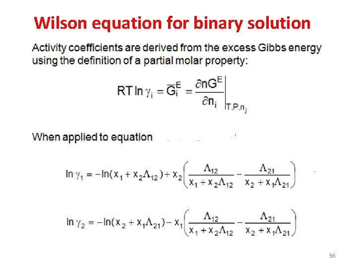
Wilson equation for binary solution 56

Wilson equation for binary solution • V 1 and V 2 – molar volumes of pure liquids at temperature. • - Energies of interaction between molecule • a - constant for a given pair of components independent of temp & prssure. 57

Wilson equation • Strength of Wilson’s approach resides in its ability to describe multi-component (3+) mixtures using binary data. – Experimental data of the mixture of interest (ie. acetone, ethanol, benzene) is not required – We only need data (or parameters) for acetoneethanol, acetone-benzene and ethanol-benzene mixtures 58

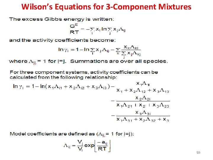
Wilson’s Equations for 3 -Component Mixtures 59

Wilson equation-advantage • Provides a good representation of VLE of a variety of miscible mixtures. – Considered the temperature dependent of the parameter – Applicable to the completely miscible system • Suitable for solutions of polar or associating components like alcohols in non-polar solvents for which the Margules and van Laar equations are generally inadequate. 60

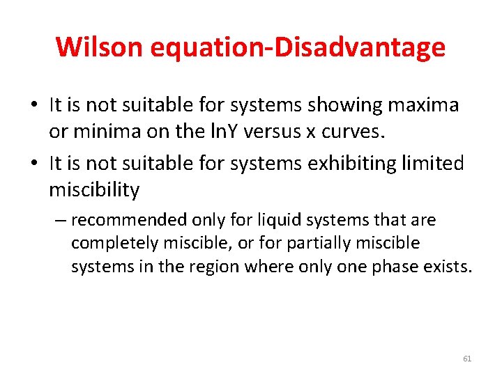
Wilson equation-Disadvantage • It is not suitable for systems showing maxima or minima on the ln. Y versus x curves. • It is not suitable for systems exhibiting limited miscibility – recommended only for liquid systems that are completely miscible, or for partially miscible systems in the region where only one phase exists. 61

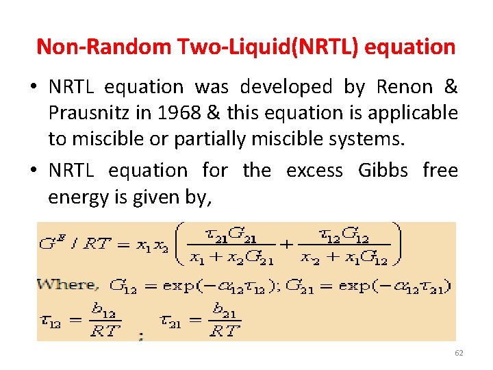
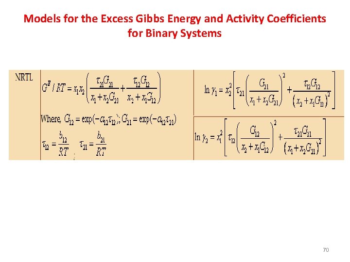
Non-Random Two-Liquid(NRTL) equation • NRTL equation was developed by Renon & Prausnitz in 1968 & this equation is applicable to miscible or partially miscible systems. • NRTL equation for the excess Gibbs free energy is given by, 62

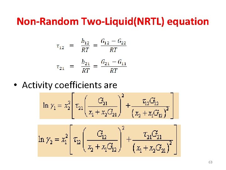
Non-Random Two-Liquid(NRTL) equation • Activity coefficients are 63

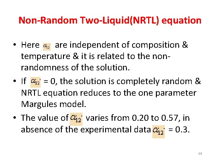
Non-Random Two-Liquid(NRTL) equation • Here are independent of composition & temperature & it is related to the nonrandomness of the solution. • If = 0, the solution is completely random & NRTL equation reduces to the one parameter Margules model. • The value of varies from 0. 20 to 0. 57, in absence of the experimental data = 0. 3. 64

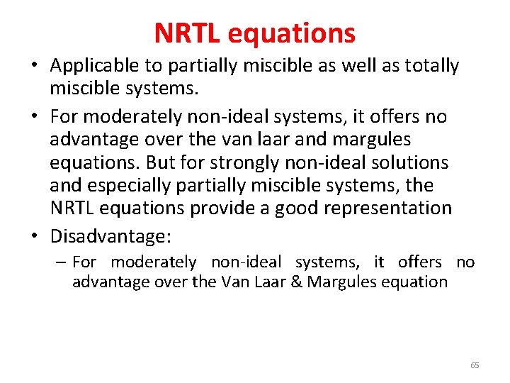
NRTL equations • Applicable to partially miscible as well as totally miscible systems. • For moderately non-ideal systems, it offers no advantage over the van laar and margules equations. But for strongly non-ideal solutions and especially partially miscible systems, the NRTL equations provide a good representation • Disadvantage: – For moderately non-ideal systems, it offers no advantage over the Van Laar & Margules equation 65

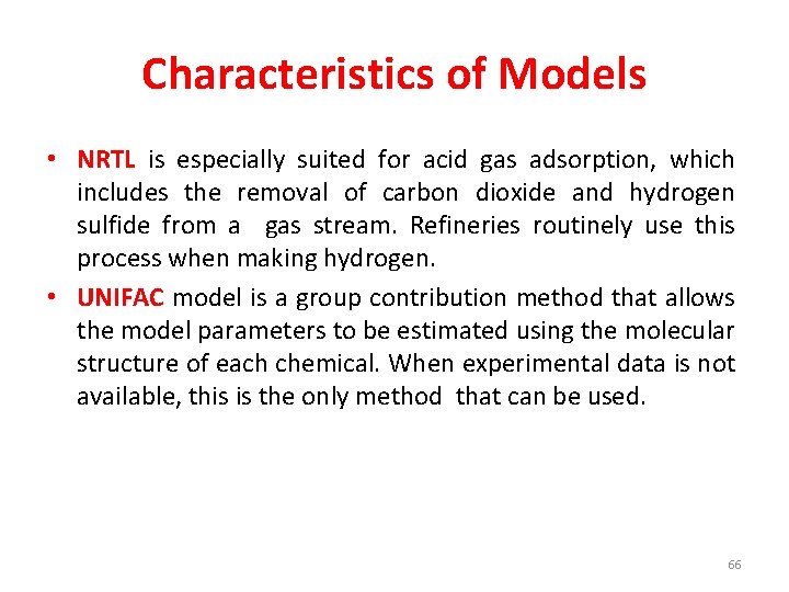
Characteristics of Models • NRTL is especially suited for acid gas adsorption, which includes the removal of carbon dioxide and hydrogen sulfide from a gas stream. Refineries routinely use this process when making hydrogen. • UNIFAC model is a group contribution method that allows the model parameters to be estimated using the molecular structure of each chemical. When experimental data is not available, this is the only method that can be used. 66

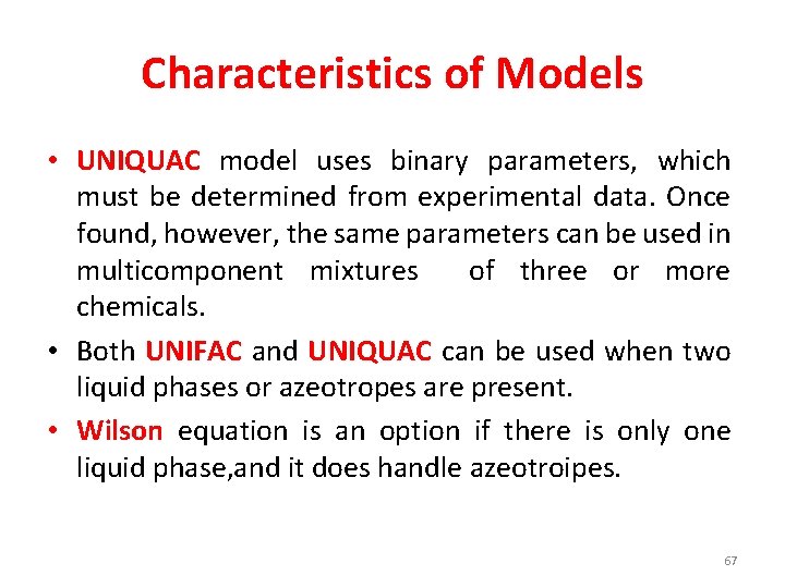
Characteristics of Models • UNIQUAC model uses binary parameters, which must be determined from experimental data. Once found, however, the same parameters can be used in multicomponent mixtures of three or more chemicals. • Both UNIFAC and UNIQUAC can be used when two liquid phases or azeotropes are present. • Wilson equation is an option if there is only one liquid phase, and it does handle azeotroipes. 67

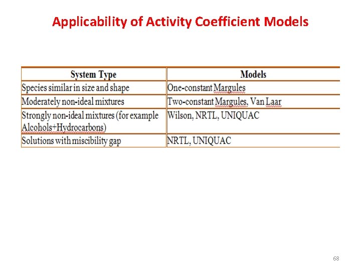
Applicability of Activity Coefficient Models 68

Models for the Excess Gibbs Energy and Activity Coefficients for Binary Systems 69

Models for the Excess Gibbs Energy and Activity Coefficients for Binary Systems 70

Relation between the model parameters and infinite dilute activity coefficients 71

72

THANK YOU