Analysis of Variance ANOVA Quantitative Methods in HPELS

Analysis of Variance (ANOVA) Quantitative Methods in HPELS 6210

Agenda Introduction n The Analysis of Variance (ANOVA) n Hypothesis Tests with ANOVA n Post Hoc Analysis n Instat n Assumptions n

Introduction n Recall There are two possible scenarios when obtaining two sets of data for comparison: ¨ Independent samples: The data in the first sample is completely INDEPENDENT from the data in the second sample. ¨ Dependent/Related samples: The two sets of data are DEPENDENT on one another. There is a relationship between the two sets of data.

Introduction n Three or more data sets? If the three or more sets of data are independent of one another Analysis of Variance (ANOVA) ¨ If the three or more sets of data are dependent on one another Repeated Measures ANOVA ¨

Introduction: Terminology Factor: Synonym of independent variable n Level: The treatment conditions that make up the factor or independent variable n Example: What is the effect of grade (1 st, 2 nd, 3 rd) on IQ? n ¨ Dependent variable: IQ ¨ Factor: Grade ¨ Levels (3): 1 st, 2 nd and 3 rd grades

Introduction: Terminology n n Between-Treatment Variance: Variance between the treatments/levels As the between-treatment variance increases: The statistic increases ¨ The p-value decreases ¨ n Greater chance of rejecting the H 0

Introduction: Terminology n n Within-Treatment Variance: Variance within the treatments/levels As the within-treatment variance increases: The statistic decreases ¨ The p-value increases ¨ n Lesser chance of rejecting the H 0

Recall the Independent-Measures t-Test n n If there was a large difference between the means (between variance) t got bigger Why? ¨t n = M 1 -M 2 / s(M 1 -M 2) The t formula can be thought of as a ratio of: ¨ Between variance (M 1 -M 2) ¨ Within variance (s(M 1 -M 2)) n Several Scenarios can occur

-Small between variance -Large within variance -t = BV / WV = near zero value Accept or reject the H 0

-Large between variance -Large within variance -t = BV / WV = near value of 1. 0 Accept or reject the H 0

-Small between variance -Small within variance -t = BV / WV = near value of 1. 0 Accept or reject the H 0

-Large between variance -Small within variance -t = BV / WV = greater than 1. 0 Accept or reject the H 0

Introduction The F-Ratio n n ANOVA is a ratio of between variance and within variance Distinction: Three or more groups

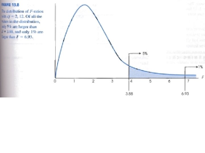
The F Distribution n n Plot all possible F-ratios F distribution There is a family of F distributions As df increases, the distribution becomes more narrow F-ratios are always positive in value ¨ Computed with two variances ¨ Variances are always positive! n n n F distribution is skewed Most values cluster around 1. 0 Figure 13. 8 (p 413)

Agenda Introduction n The Analysis of Variance (ANOVA) n Hypothesis Tests with ANOVA n Post Hoc Analysis n Instat n Assumptions n

ANOVA n Statistical Notation: ¨k = number of treatment conditions (levels) ¨ nx = number of samples per treatment level ¨ N = total number of samples n N = kn if sample sizes are equal = SX for any given treatment level ¨ G = ST ¨ MS = mean square = variance ¨ Tx

ANOVA n Formula Considerations: = ST 2/n – G 2/N ¨ SSwithin = SSSinside each treatment ¨ SStotal = SSwithin + SSbetween ¨ SSbetween n SStotal = SX 2 – G 2/N

ANOVA n Formula Considerations: ¨ dftotal =N– 1 ¨ dfbetween = k – 1 ¨ dfwithin = S(n – 1) n dfwithin = Sdfin each treatment

ANOVA n Formula Considerations: ¨ MSbetween = s 2 between = SSbetween / dfbetween ¨ MSwithin = s 2 within = SSwithin / dfwithin ¨ F = MSbetween / MSwithin

Independent-Measures Designs n Static-Group Comparison Design: Administer treatment to two or more groups and perform posttest ¨ Perform posttest to control group ¨ Compare groups ¨ X 1 O X 2 O O

Independent-Measures Designs n Quasi-Experimental Pretest Posttest Control Group Design: Perform pretest on three or more groups ¨ Administer treatments to treatment groups ¨ Perform posttests on all groups ¨ Compare delta (Δ) scores ¨ O X 1 O Δ O X 2 O Δ O

Independent-Measures Designs n Randomized Pretest Posttest Control Group Design: ¨ ¨ ¨ Randomly select subjects from three or more populations Perform pretest on all groups Administer treatments to treatment groups Perform posttests on all groups Compare delta (Δ) scores R O X 1 O Δ R O X 2 O Δ R O O Δ

Agenda Introduction n The Analysis of Variance (ANOVA) n Hypothesis Tests with ANOVA n Post Hoc Analysis n Instat n Assumptions n

Hypothesis Test: ANOVA n n Example 13. 1 (p 415) Overview: ¨ Researchers are interested in the effectiveness different pain relievers (A, B and C) compared placebo (D) ¨ N = 20 randomly assigned to the four treatments (n = 5) ¨ Amount of time (s) each subject could withstand a painfully hot stimulus was measured

Hypothesis Test: ANOVA n Questions: ¨ What is the experimental design? ¨ What is the independent variable/factor? ¨ How many levels are there? ¨ What is the dependent variable?

Step 1: State Hypotheses Non-Directional H 0 : µA = µB = µC = µD H 1: At least one mean is different than the others Directional? Too many too list Step 2: Set Criteria Alpha (a) = 0. 05 Critical Value: Use F Distribution Table Appendix B. 4 (p 693) Information Needed: dfbetween = k – 1 dfwithin = S(n – 1)

Step 3: Collect Data and Calculate Statistic Total Sum of Squares Between SStotal = SX 2 – G 2/N SSbetween = ST 2/n – SG 2/N SStotal = 262 – 602/20 SSbetween = 52/5+102/5+252/5 – 602/20 SStotal = 262 - 180 SSbetween = (5+20+80+125) - 180 SStotal = 82 SSbetween = 50 Sum of Squares Within SSwithin = SSSinside each treatment SSwithin = 8+8+6+10 SSwithin = 32

Step 3: Collect Data and Calculate Statistic F-Ratio Mean Square Between F = 16. 67 / 2 MSbetween = SSbetween / dfbetween F = 8. 33 MSbetween = 50 / 3 MSbetween = 16. 67 Mean Square Within MSwithin = SSwithin / dfwithin MSwithin = 32/16 MSwithin = 2 F = MSbetween / MSwithin Step 4: Make Decision

Agenda Introduction n The Analysis of Variance (ANOVA) n Hypothesis Tests with ANOVA n Post Hoc Analysis n Instat n Assumptions n

Post Hoc Analysis n What ANOVA tells us: ¨ Rejection of the H 0 tells you that there is a high PROBABILITY that AT LEAST ONE difference exists SOMEWHERE n What ANOVA doesn’t tell us: ¨ Where n the differences lie Post hoc analysis is needed to determine which mean(s) is(are) different

Post Hoc Analysis Post Hoc Tests: Additional hypothesis tests performed after a significant ANOVA test to determine where the differences lie. n Post hoc analysis IS NOT PERFORMED unless the initial ANOVA H 0 was rejected! n

Post Hoc Analysis Type I Error n n n Type I error: Rejection of a true H 0 Pairwise comparisons: Multiple post hoc tests comparing the means of all “pairwise combinations” Problem: Each post hoc hypothesis test has chance of type I error As multiple tests are performed, the chance of type I error accumulates Experimentwise alpha level: Overall probability of type I error that accumulates over a series of pairwise post hoc hypothesis tests How is this accumulation of type I error controlled?

Two Methods n Bonferonni or Dunn’s Method: ¨ Perform multiple t-tests of desired comparisons or contrasts ¨ Make decision relative to a / # of tests ¨ This reduction of alpha will control for the inflation of type I error n Specific post hoc tests: ¨ Note: There are many different post hoc tests that can be used ¨ Our book only covers two (Tukey and Scheffe)

Tukey’s Honestly Significant Difference (HSD) Test n Overview: ¨ Computes a single value that determines the minimum difference (HSD) between any two means necessary for rejection of the H 0 ¨ Compares the HSD value to all of the contrast results ¨ If the contrast result exceeds the HSD, the H 0 of that particular contrast is rejected

Tukey’s HSD Calculation Formulas: n Equal sample sizes n ¨ HSD n = q√MSwithin / n Unequal sample sizes ¨ HSD = q√(MSwithin/2)(1/n 1+1/n 2)

Tukey’s HSD Calculations n n Formula Considerations: q = value found in Table B. 5 (p 696) ¨ Left column: dfwithin ¨ Top row: k treatments ¨ Body: n n Regular font: a = 0. 05 Bold font: a = 0. 01 ¨ MSwithin = value from ANOVA calculation ¨ n = number of subjects in each treatment n Example 13. 5 (p 427)

Step 1: State Hypotheses Step 2: Set Criteria Null Alpha (a) = 0. 05 H 0 : µA = µB Step 3: Calculate Statistic H 0 : µA = µC Get q from Table B. 5 H 0 : µB = µC Information needed: Alternative dfwithin = 24 H 1 : µA µB k=3 H 1 : µA µC a= 0. 05 H 1 : µB µC q = 3. 53

Table 13. 6 Calculate Tukey’s HSD Value HSD = q MSwithin / n HSD = 3. 53 4 / 9 HSD = 2. 36 Step 4: Make Decision: A significantly greater than B MA – MB = 2. 44 > 2. 36 A significantly greater than C MA – MC = 4. 00 > 2. 36 B not significantly different than C MB – MC = 1. 56 < 2. 36

Scheffe n Overview: ¨ Most conservative/cautious of all post hoc tests ¨ Uses an F-ratio (like ANOVA) on only two treatments n Controls for type I error: ¨ Uses k value from the original ANOVA thus the numerator of the F-ratio for the Scheffe test is k – 1 ¨ Uses same critical value used for the ANOVA n Calculation of Scheffe is identical to the ANOVA however: ¨ SSbetween n uses the two means of interest Example 13. 6 (p 428)

Step 1: State Hypotheses Step 3: Calculate Statistic Null Sum of squares between: H 0 : µA = µB SSbetween = ST 2/n – G 2/N H 0 : µA = µC SSbetween = (272/9 + 492/9) – 762/18 H 0 : µB = µC SSbetween = (81+266. 78) – 320. 89 Alternative SSbetween = 26. 89 H 1 : µA µB H 1 : µA µC H 1 : µB µC Step 2: Set Criteria Alpha (a) = 0. 05 Critical Value 3. 40 dfbetween = 2 dfwithin = 24 a = 0. 05 SSwithin from original ANOVA = 96 Mean square between and within MSbetween = SSbetween/dfbetween MSbetween = 26. 89 / 2 = 13. 45 MSwithin from original ANOVA = 4 F = MSbetween / MSwithin F = 13. 45 / 4 F = 3. 36

F = MSbetween / MSwithin F = 13. 45 / 4 F = 3. 36 df = 2, 24 Step 4: Make Decision F = 3. 36 < 3. 40 (critical value) Accept or reject? Repeat for the other two contrasts: H 0 : µA = µC H 0 : µB = µC 3. 40

Agenda Introduction n The Analysis of Variance (ANOVA) n Hypothesis Tests with ANOVA n Post Hoc Analysis n Instat n Assumptions n

Instat Type dependent variable data from the three or more samples into one column: n Label column appropriately ¨ In a second column, type in the grouping variable (independent variable) next to each data point: n Label column appropriately Convert the grouping column into a “factor” column: ¨ ¨ n n n n Highlight the grouping column. Choose “Manage” Choose “Column Properties” Choose “Factor” Select the appropriate column to be converted Indicate the number of levels in the factor Click OK

Instat Choose “Statistics” n Choose “Analysis of Variance” Choose “One-Way” Y-Variate: ¨ ¨ ¨ n Factor: ¨ n Choose the factor column or grouping/independent variable Plots: ¨ n ¨ ¨ Choose the dependent variable Not necessary to choose any Click OK. Interpret the p-value!!! Post Hoc Analysis: n ¨ Perform multiple Independent-Measures t-Tests with the Bonferonni/Dunn correction method

Reporting ANOVA Results n Information to include: Value of the F statistic ¨ Degrees of freedom: ¨ n n ¨ n Between: k – 1 Within: S(n – 1) p-value Examples: ¨ A significant treatment effect was observed (F(2, 24) = 8. 33, p = 0. 02)

Reporting ANOVA Results n An ANOVA summary table is often included Source SS df MS Between 50 3 16. 67 Within 32 16 2 Total 82 19 F = 8. 33

Agenda Introduction n The Analysis of Variance (ANOVA) n Hypothesis Tests with ANOVA n Post Hoc Analysis n Instat n Assumptions n

Assumptions of ANOVA Independent Observations n Normal Distribution n Scale of Measurement n ¨ Interval n or ratio Equal variances (homogeneity)

Violation of Assumptions Nonparametric Version Kruskall-Wallis Test (Chapter 17) n When to use the Kruskall-Wallis Test: n ¨ Independent-Measures design with three or more groups ¨ Scale of measurement assumption violation: n Ordinal data ¨ Normality n assumption violation: Regardless of scale of measurement

Textbook Assignment n Problems: 3, 5, 17 a, 21