Analysis of Variance ANOVA Anwar Ahmad ANOVA Samples

Analysis of Variance ANOVA Anwar Ahmad

ANOVA • Samples from different populations (treatment groups) • Any difference among the population means? • Null hypothesis: no difference among the means

ANOVA Examples • Effect of different lots of vaccine on antibody titer • Effect of different measurement techniques on serum cholesterol determination from the same pool of serum

ANOVA Examples • Water samples drawn at various location in a city • Effect of antihypertensive drugs and placebo on mean systolic blood pressure

ANOVA • Partitioning of the sum of squares • The fundamental technique is a partitioning of the total sum of squares into components related to the effects used in the model.

Analysis of Variance ANOVA is a technique to differentiate between sample means to draw inferences about the presence or absence of variations between populations means.

ANOVA • The key statistic in ANOVA is the F-test of difference of group means, testing if the means of the groups formed by values of the independent variable (or combinations of values for multiple independent variables) are different enough not to have occurred by chance.

ANOVA • If the group means do not differ significantly then it is inferred that the independent variable(s) did not have an effect on the dependent variable. • If the F test shows that overall the independent variable(s) is (are) related to the dependent variable, then multiple comparison tests of significance are used to explore just which values of the independent(s) have the most to do with the relationship.

ANOVA • The overall test for differences among means. • Used when we wish to determine significance among two or more means. Ho = m 1= m 2 = m 3 = Mk.

Analysis of Variance • Analysis of variance is a technique for testing the null hypothesis that one or more samples were drawn at random from the same population. • Like “t” or “z” the analysis of variance provides us with a test of significance. • The “F” test provides an estimate of the experimental effect and an estimate of the error terms.

Analysis of Variance • A procedure for determining how much of the total variability among scores to attribute to various sources of variation and for testing hypotheses concerning some of the sources.

Analysis of Variance • A ratio is then made of the two independent variance estimates. This ratio is then compared with the critical f-ratio found in the F table.

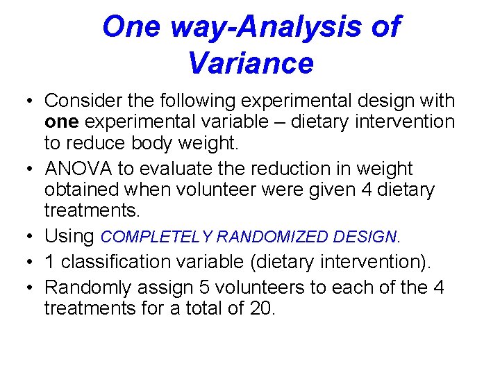
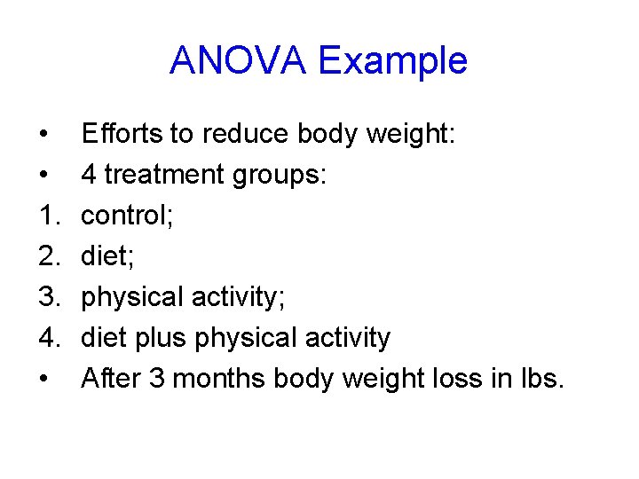
One way-Analysis of Variance • Consider the following experimental design with one experimental variable – dietary intervention to reduce body weight. • ANOVA to evaluate the reduction in weight obtained when volunteer were given 4 dietary treatments. • Using COMPLETELY RANDOMIZED DESIGN. • 1 classification variable (dietary intervention). • Randomly assign 5 volunteers to each of the 4 treatments for a total of 20.

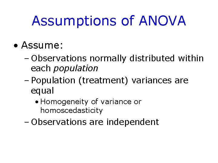
Assumptions of ANOVA • Assume: – Observations normally distributed within each population – Population (treatment) variances are equal • Homogeneity of variance or homoscedasticity – Observations are independent

Assumptions--cont. • Analysis of variance is generally robust – A robust test is one that is not greatly affected by violations of assumptions.

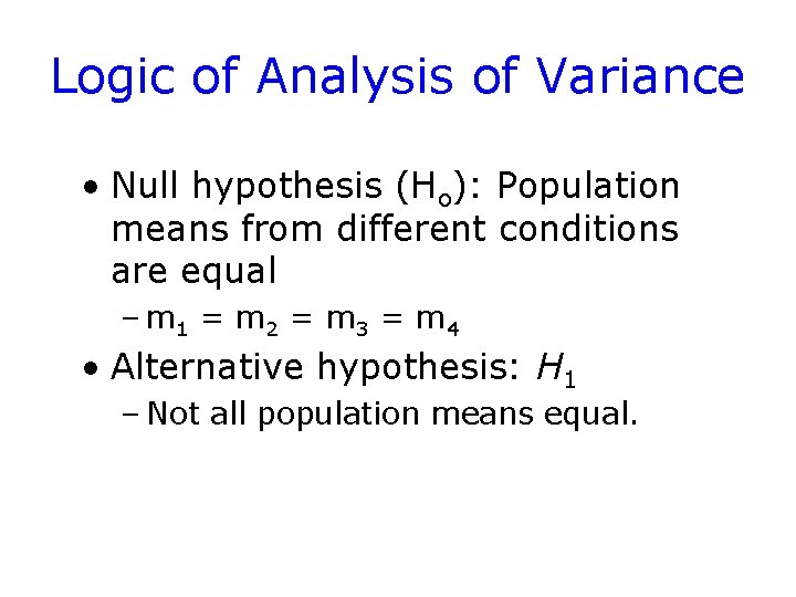
Logic of Analysis of Variance • Null hypothesis (Ho): Population means from different conditions are equal – m 1 = m 2 = m 3 = m 4 • Alternative hypothesis: H 1 – Not all population means equal.

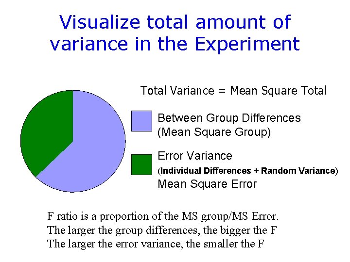
Visualize total amount of variance in the Experiment Total Variance = Mean Square Total Between Group Differences (Mean Square Group) Error Variance (Individual Differences + Random Variance) Mean Square Error F ratio is a proportion of the MS group/MS Error. The larger the group differences, the bigger the F The larger the error variance, the smaller the F

Logic--cont. • Create a measure of variability among treatment group means – MSgroup • Create a measure of variability within treatment groups – MSerror

Logic--cont. • Form ratio of MSgroup /MSerror – Ratio approximately 1 if null true – Ratio significantly larger than 1 if null false

Calculations • Sum of Squares (SS) • SStotal • SSgroups • SSerror • Compute degrees of freedom (df ) • Compute mean squares and F-ratio Cont.

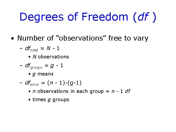
Degrees of Freedom (df ) • Number of “observations” free to vary – dftotal = N - 1 • N observations – dfgroups = g - 1 • g means – dferror = (n - 1)-(g-1) • n observations in each group = n - 1 df • times g groups

ANOVA Example • • 1. 2. 3. 4. • Efforts to reduce body weight: 4 treatment groups: control; diet; physical activity; diet plus physical activity After 3 months body weight loss in lbs.

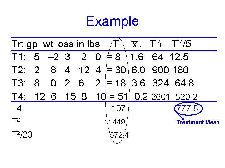
Example Trt gp wt loss in lbs Ti xi. T 2 i/5 T 1: 5 – 2 3 2 0 = 8 1. 6 64 12. 5 T 2: 2 8 4 12 4 = 30 6. 0 900 180 T 3: 8 0 2 6 2 = 18 3. 6 324 64. 8 T 4: 12 6 15 8 10 = 51 0. 2 2601 520. 2 4 T 2/20 107 11449 572. 4 777. 8 Treatment Mean

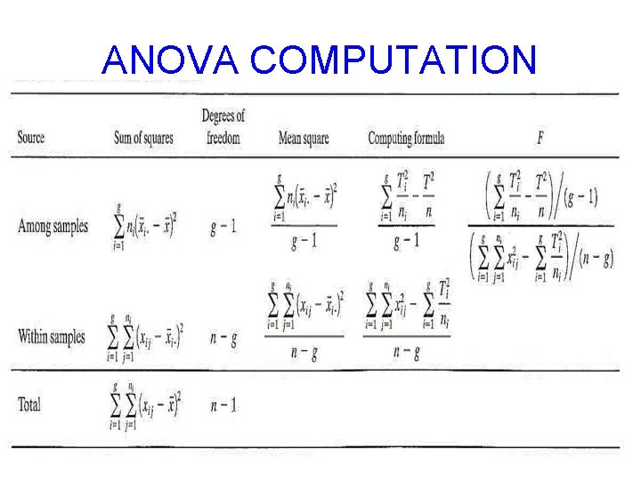
ANOVA COMPUTATION

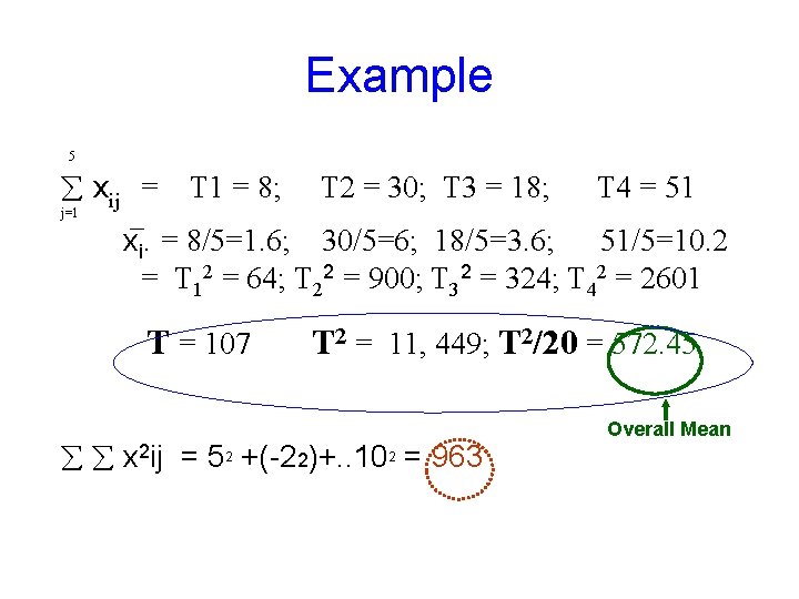
Example 5 xij = T 1 = 8; T 2 = 30; T 3 = 18; T 4 = 51 j=1 xi. = 8/5=1. 6; 30/5=6; 18/5=3. 6; 51/5=10. 2 = T 12 = 64; T 22 = 900; T 32 = 324; T 42 = 2601 T = 107 2 = 11, 449; T 2/20 = 572. 45 T x 2 ij = 52 +(-22)+. . 102 = 963 Overall Mean

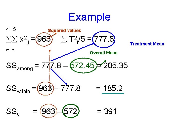
Example 4 5 Squared values x 2 ij = 963 T 2 i/5 = 777. 8 i=1 Overall Mean SSamong = 777. 8 – 572. 45 = 205. 35 SSwithin = 963 – 777. 8 = 185. 2 SSy = 391 = 963 – 572 Treatment Mean

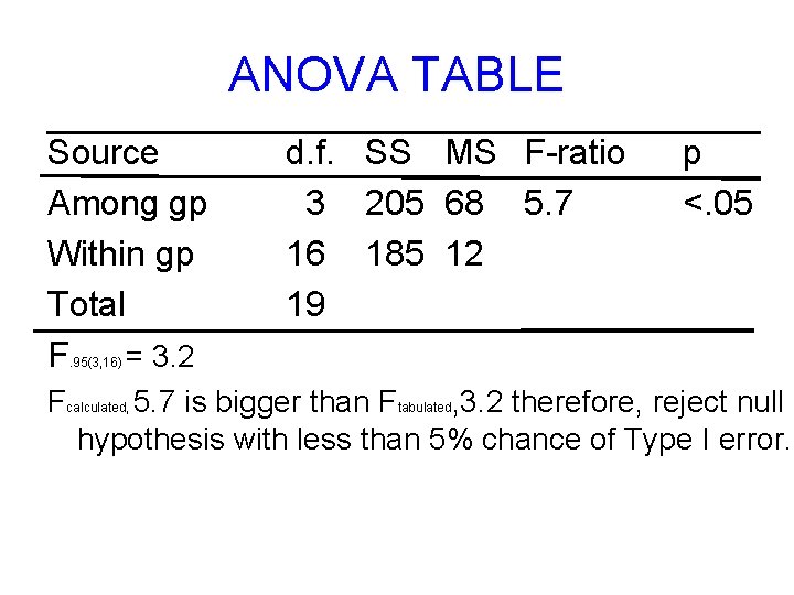
ANOVA TABLE Source Among gp Within gp Total F = 3. 2 d. f. SS MS F-ratio 3 205 68 5. 7 16 185 12 19 p <. 05 . 95(3, 16) Fcalculated, 5. 7 is bigger than Ftabulated, 3. 2 therefore, reject null hypothesis with less than 5% chance of Type I error.

When there are more than two groups • Significant F only shows that not all groups are equal – what groups are different? ? ? – Food for Thought

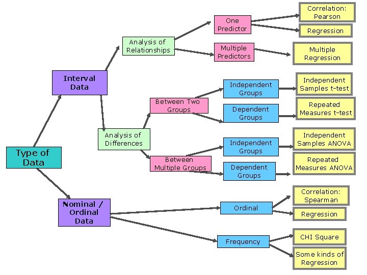
One Predictor Analysis of Relationships Interval Data Independent Groups Between Two Groups Analysis of Differences Type of Data Dependent Groups Independent Groups Between Multiple Groups Nominal / Ordinal Data Multiple Predictors Dependent Groups Correlation: Pearson Regression Multiple Regression Independent Samples t-test Repeated Measures t-test Independent Samples ANOVA Repeated Measures ANOVA Correlation: Spearman Ordinal Frequency Regression CHI Square Some kinds of Regression

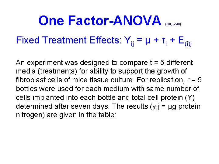
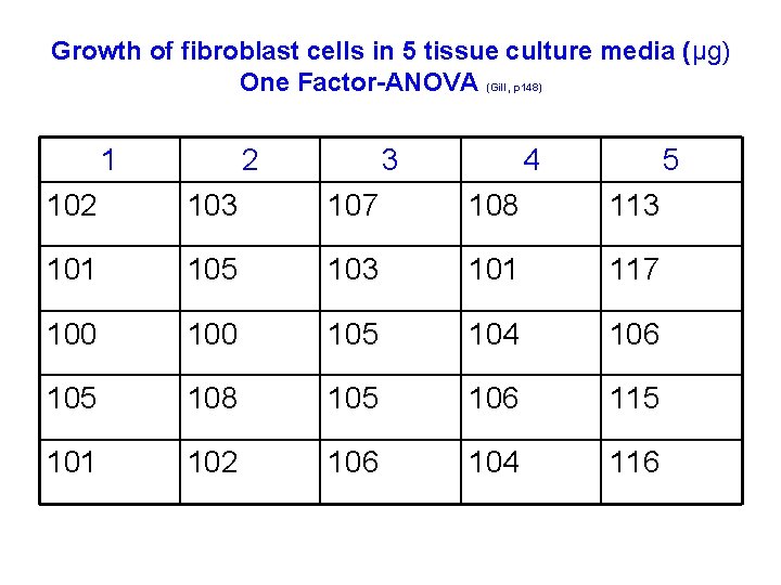
One Factor-ANOVA (Gill, p 148) Fixed Treatment Effects: Yij = μ + τi + E(i)j An experiment was designed to compare t = 5 different media (treatments) for ability to support the growth of fibroblast cells of mice tissue culture. For replication, r = 5 bottles were used for each medium with same number of cells implanted into each bottle and total cell protein (Y) determined after seven days. The results (yij = μg protein nitrogen) are given in the table:

Growth of fibroblast cells in 5 tissue culture media (μg) One Factor-ANOVA (Gill, p 148) 1 2 3 4 5 102 103 107 108 113 101 105 103 101 117 100 105 104 106 105 108 105 106 115 101 102 106 104 116

One Factor-ANOVA • SSy = (1022 +1012 +…+1162) – [102+101+… 116)2/25] = 279, 985 – 279, 418 = 567 • SST = [(102+101+… 101)2/5 +(103+105+…+102) 2/5+…] = 279, 820 – 279, 418 = 402 • SSE = 567 – 402 = 165 (Gill, p 148)

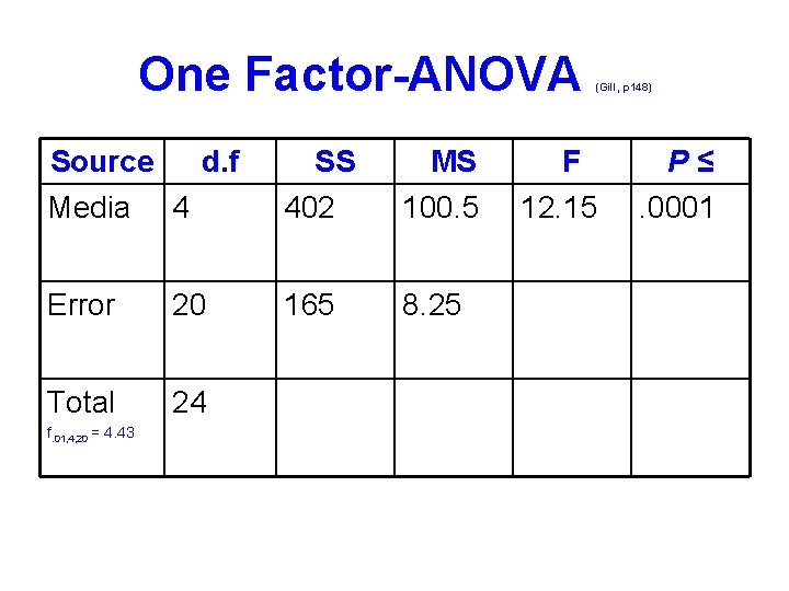
One Factor-ANOVA Source d. f Media 4 SS 402 MS 100. 5 Error 20 165 8. 25 Total 24 f. 01, 4, 20 = 4. 43 (Gill, p 148) F 12. 15 P≤. 0001

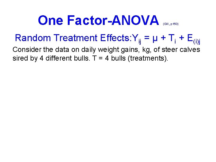
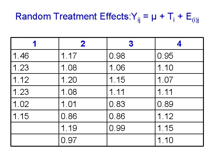
One Factor-ANOVA (Gill, p 150) Random Treatment Effects: Yij = μ + Ti + E(i)j Consider the data on daily weight gains, kg, of steer calves sired by 4 different bulls. T = 4 bulls (treatments).

Random Treatment Effects: Yij = μ + Ti + E(i)j 1 1. 46 1. 23 1. 12 1. 23 1. 02 1. 15 2 1. 17 1. 08 1. 20 1. 08 1. 01 0. 86 1. 19 0. 97 3 0. 98 1. 06 1. 15 1. 11 0. 83 0. 86 0. 99 4 0. 95 1. 10 1. 07 1. 11 0. 89 1. 12 1. 15 1. 10

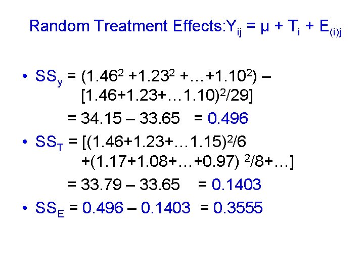
Random Treatment Effects: Yij = μ + Ti + E(i)j • SSy = (1. 462 +1. 232 +…+1. 102) – [1. 46+1. 23+… 1. 10)2/29] = 34. 15 – 33. 65 = 0. 496 • SST = [(1. 46+1. 23+… 1. 15)2/6 +(1. 17+1. 08+…+0. 97) 2/8+…] = 33. 79 – 33. 65 = 0. 1403 • SSE = 0. 496 – 0. 1403 = 0. 3555

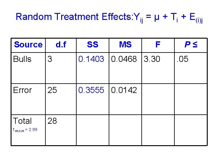
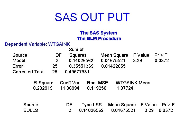
Random Treatment Effects: Yij = μ + Ti + E(i)j Source d. f SS MS F Bulls 3 0. 1403 0. 0468 3. 30 Error 25 0. 3555 0. 0142 Total 28 f. 05, 3, 25 = 2. 99 P≤. 05

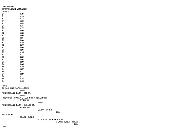
Data STEER; INPUT BULLS $ WTGAINK; CARDS; B 1 1. 46 B 1 1. 23 B 1 1. 12 B 1 1. 23 B 1 1. 02 B 1 1. 15 B 2 1. 17 B 2 1. 08 B 2 1. 20 B 2 1. 08 B 2 1. 01 B 2 0. 86 B 2 1. 19 B 2 0. 97 B 3 0. 98 B 3 1. 06 B 3 1. 15 B 3 1. 11 B 3 0. 83 B 3 0. 86 B 3 0. 99 B 4 0. 95 B 4 1. 10 B 4 1. 07 B 4 1. 11 B 4 0. 89 B 4 1. 12 B 4 1. 15 B 4 1. 10 ; RUN; PROC PRINT DATA = STEER; RUN; PROC MEANS DATA = STEER; RUN; PROC SORT DATA = STEER OUT = BULLSORT; BY BULLS; RUN; PROC MEANS DATA = BULLSORT; BY BULLS; VAR WTGAINK; RUN; PROC GLM; CLASS BULLS; MODEL WTGAINK = BULLS; MEANS BULLS/TUKEY; RUN; QUIT;

SAS OUT PUT The SAS System The GLM Procedure Dependent Variable: WTGAINK Sum of Source DF Squares Model 3 0. 14026562 Error 25 0. 35551369 Corrected Total 28 0. 49577931 R-Square 0. 282919 Source BULLS Coeff Var 11. 06994 DF 3 Mean Square 0. 04675521 0. 01422055 Root MSE 0. 119250 F Value 3. 29 Pr > F 0. 0372 WTGAINK Mean 1. 077241 Type I SS Mean Square 0. 14026562 0. 04675521 F Value Pr > F 3. 29 0. 0372

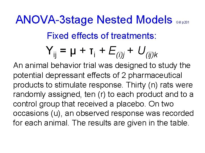
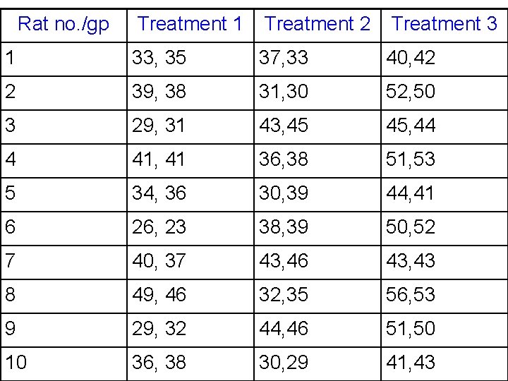
ANOVA-3 stage Nested Models Gill p 201 Fixed effects of treatments: Yij = μ + τi + E(i)j + U(ij)k An animal behavior trial was designed to study the potential depressant effects of 2 pharmaceutical products to stimulate response. Thirty (n) rats were randomly assigned, ten (r) to each product and to a control group that received a placebo. On two occasions (u), an observed response was recorded for each animal. The results are given in the table.

Rat no. /gp Treatment 1 Treatment 2 Treatment 3 1 33, 35 37, 33 40, 42 2 39, 38 31, 30 52, 50 3 29, 31 43, 45 45, 44 4 41, 41 36, 38 51, 53 5 34, 36 30, 39 44, 41 6 26, 23 38, 39 50, 52 7 40, 37 43, 46 43, 43 8 49, 46 32, 35 56, 53 9 29, 32 44, 46 51, 50 10 36, 38 30, 29 41, 43

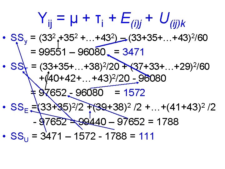
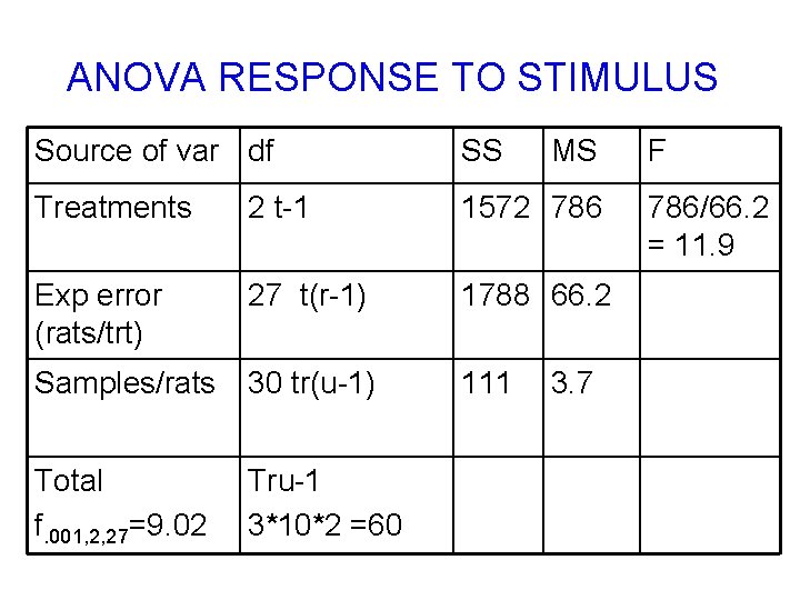
Yij = μ + τi + E(i)j + U(ij)k • SSy = (332 +352 +…+432) – (33+35+…+43)2/60 = 99551 – 96080 = 3471 • SST = (33+35+…+38)2/20 + (37+33+…+29)2/60 +(40+42+…+43)2/20 - 96080 = 97652 - 96080 = 1572 • SSE =(33+35)2/2 +(39+38)2 /2 +…+(41+43)2 /2 - 97652 = 99440 – 97652 = 1788 • SSU = 3471 – 1572 - 1788 = 111

ANOVA RESPONSE TO STIMULUS Source of var df SS MS Treatments 2 t-1 1572 786 Exp error (rats/trt) 27 t(r-1) 1788 66. 2 Samples/rats 30 tr(u-1) 111 Total f. 001, 2, 27=9. 02 Tru-1 3*10*2 =60 3. 7 F 786/66. 2 = 11. 9

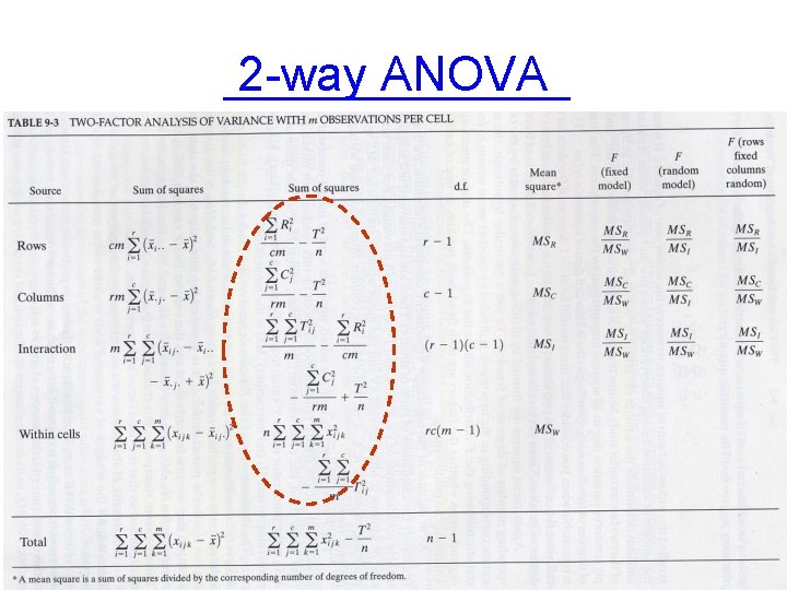
2 -way ANOVA

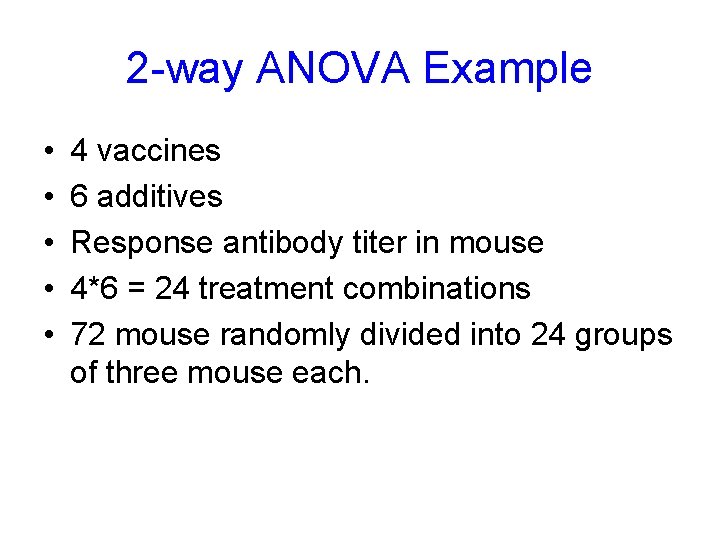
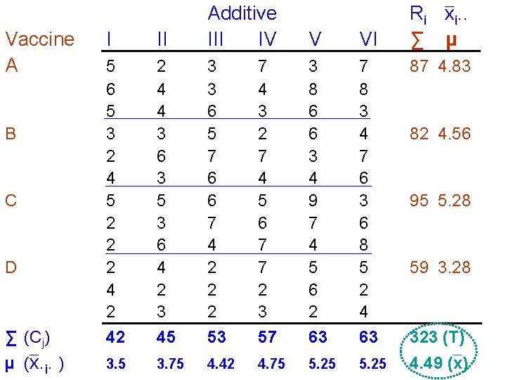
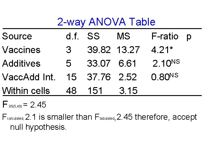
2 -way ANOVA Example • • • 4 vaccines 6 additives Response antibody titer in mouse 4*6 = 24 treatment combinations 72 mouse randomly divided into 24 groups of three mouse each.

I II Additive III IV 5 6 5 3 2 4 5 2 2 2 4 4 3 6 3 5 3 6 4 2 3 3 3 6 5 7 6 6 7 4 2 2 2 7 4 3 2 7 4 5 6 7 7 2 3 3 8 6 6 3 4 9 7 4 5 6 2 7 8 3 4 7 6 3 6 8 5 2 4 87 4. 83 ∑ (Cj) 42 45 53 57 63 63 323 (T) µ (x. i. ) 3. 5 3. 75 4. 42 4. 75 5. 25 4. 49 (x) Vaccine A B C D V VI Ri xi. . ∑ µ 82 4. 56 95 5. 28 59 3. 28

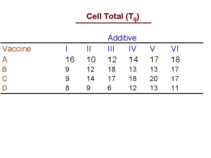
Cell Total (Tij) Vaccine A I 16 II 10 Additive III IV 12 14 B C D 9 9 8 12 14 9 18 17 6 13 18 12 V 17 VI 18 13 20 13 17 17 11

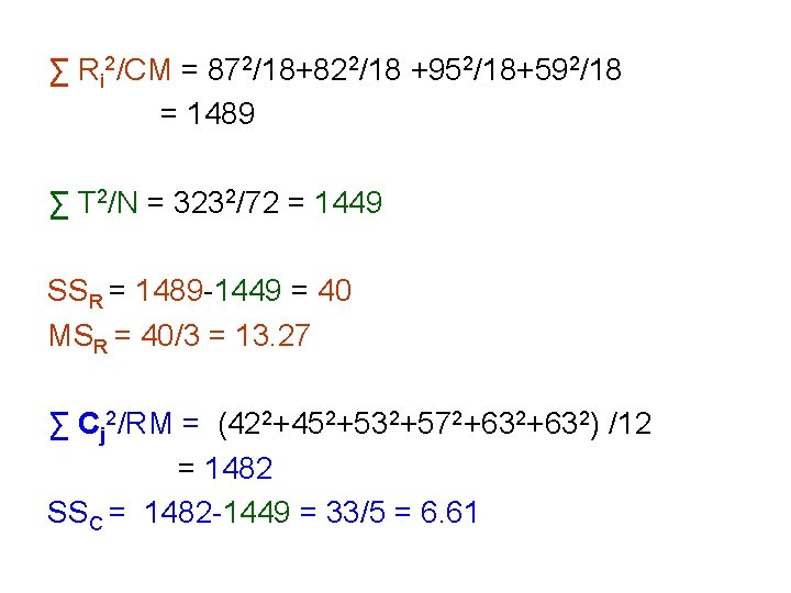
∑ Ri 2/CM = 872/18+822/18 +952/18+592/18 = 1489 ∑ T 2/N = 3232/72 = 1449 SSR = 1489 -1449 = 40 MSR = 40/3 = 13. 27 ∑ Cj 2/RM = (422+452+532+572+632) /12 = 1482 SSC = 1482 -1449 = 33/5 = 6. 61

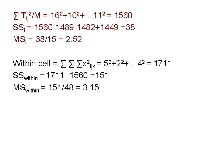
∑ Tij 2/M = 162+102+… 112 = 1560 SSI = 1560 -1489 -1482+1449 =38 MSI = 38/15 = 2. 52 Within cell = ∑ ∑ ∑x 2 ijk = 52+22+… 42 = 1711 SSwithin = 1711 - 1560 =151 MSwithin = 151/48 = 3. 15

2 -way ANOVA Table Source Vaccines Additives Vacc. Add Int. Within cells F = 2. 45 d. f. 3 5 15 48 SS 39. 82 33. 07 37. 76 151 MS 13. 27 6. 61 2. 52 3. 15 F-ratio p 4. 21* 2. 10 NS 0. 80 NS . 95(5, 48) Fcalculated, 2. 1 is smaller than Ftabulated, 2. 45 therefore, accept null hypothesis.

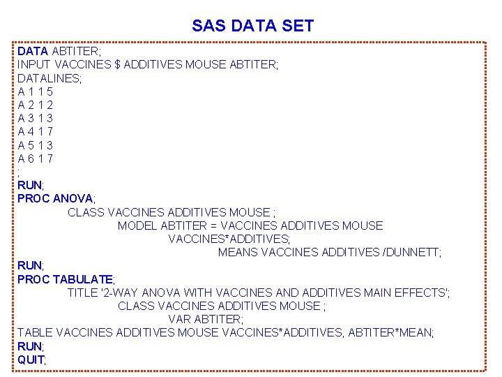
SAS DATA SET DATA ABTITER; INPUT VACCINES $ ADDITIVES MOUSE ABTITER; DATALINES; A 115 A 212 A 313 A 417 A 513 A 617 ; RUN; PROC ANOVA; CLASS VACCINES ADDITIVES MOUSE ; MODEL ABTITER = VACCINES ADDITIVES MOUSE VACCINES*ADDITIVES; MEANS VACCINES ADDITIVES /DUNNETT; RUN; PROC TABULATE; TITLE '2 -WAY ANOVA WITH VACCINES AND ADDITIVES MAIN EFFECTS'; CLASS VACCINES ADDITIVES MOUSE ; VAR ABTITER; TABLE VACCINES ADDITIVES MOUSE VACCINES*ADDITIVES, ABTITER*MEAN; RUN; QUIT;

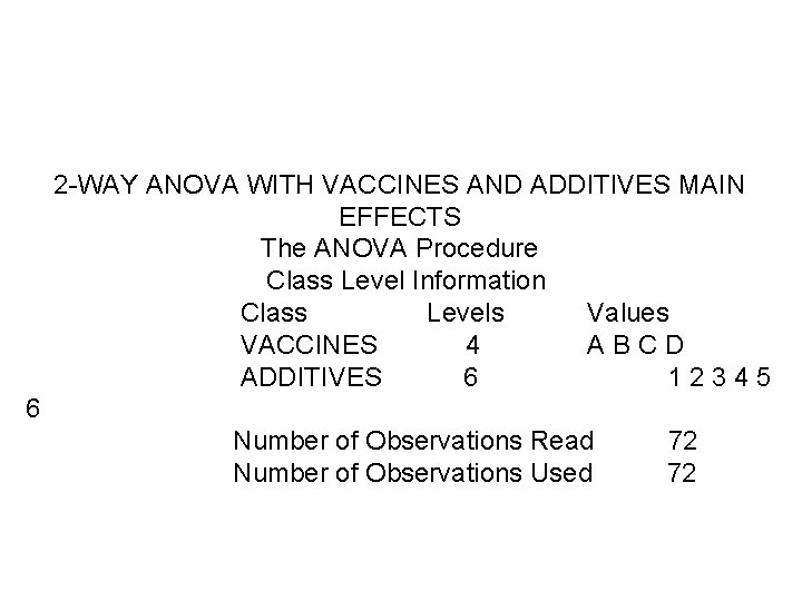
2 -WAY ANOVA WITH VACCINES AND ADDITIVES MAIN EFFECTS The ANOVA Procedure Class Level Information Class Levels Values VACCINES 4 ABCD ADDITIVES 6 12345 6 Number of Observations Read Number of Observations Used 72 72

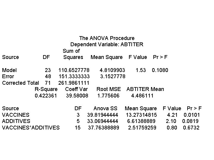
Source DF The ANOVA Procedure Dependent Variable: ABTITER Sum of Squares Mean Square F Value Model 23 110. 6527778 Error 48 151. 3333333 Corrected Total 71 261. 9861111 R-Square Coeff Var 0. 422361 39. 58008 Source VACCINES ADDITIVES VACCINES*ADDITIVES DF 3 5 15 4. 8109903 3. 1527778 Root MSE 1. 775606 Anova SS 39. 81944444 33. 06944444 37. 76388889 1. 53 Pr > F 0. 1080 ABTITER Mean 4. 486111 Mean Square 13. 27314815 6. 61388889 2. 51759259 F Value Pr > F 4. 21 0. 0101 2. 10 0. 0819 0. 80 0. 6732

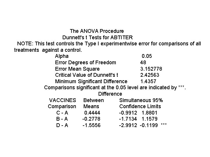
The ANOVA Procedure Dunnett's t Tests for ABTITER NOTE: This test controls the Type I experimentwise error for comparisons of all treatments against a control. Alpha 0. 05 Error Degrees of Freedom 48 Error Mean Square 3. 152778 Critical Value of Dunnett's t 2. 42563 Minimum Significant Difference 1. 4357 Comparisons significant at the 0. 05 level are indicated by ***. Difference VACCINES Between Simultaneous 95% Comparison Means Confidence Limits C-A 0. 4444 -0. 9912 1. 8801 B-A -0. 2778 -1. 7134 1. 1579 D-A -1. 5556 -2. 9912 -0. 1199 ***

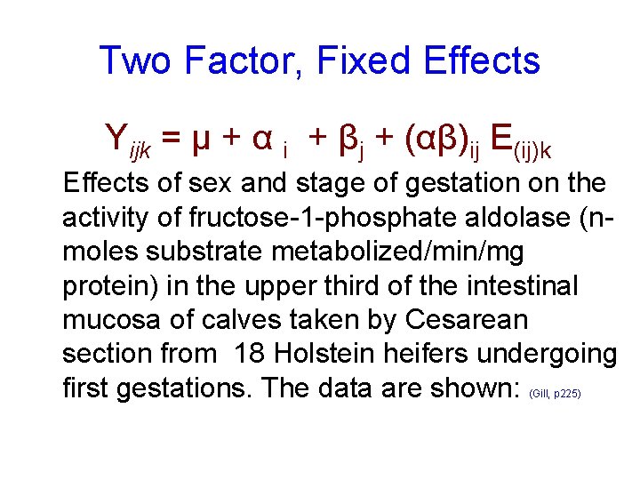
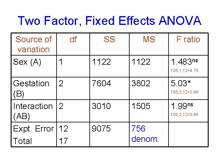
Two Factor, Fixed Effects Yijk = μ + α i + βj + (αβ)ij E(ij)k Effects of sex and stage of gestation on the activity of fructose-1 -phosphate aldolase (nmoles substrate metabolized/min/mg protein) in the upper third of the intestinal mucosa of calves taken by Cesarean section from 18 Holstein heifers undergoing first gestations. The data are shown: (Gill, p 225)

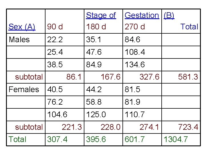
Sex (A) 90 d Stage of 180 d Males 22. 2 35. 1 84. 6 25. 4 47. 6 108. 4 38. 5 84. 9 134. 6 subtotal Females subtotal Total 86. 1 167. 6 Gestation (B) 270 d Total 327. 6 40. 5 44. 2 81. 5 76. 2 58. 8 81. 9 104. 6 125. 0 110. 7 221. 3 307. 4 228. 0 395. 6 274. 1 601. 7 581. 3 723. 4 1304. 7

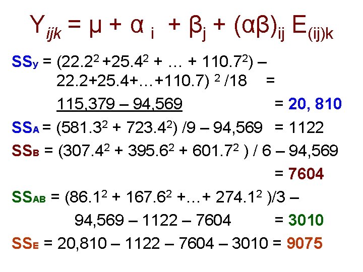
Yijk = μ + α i + βj + (αβ)ij E(ij)k SSy = (22. 22 +25. 42 + … + 110. 72) – 22. 2+25. 4+…+110. 7) 2 /18 = 115, 379 – 94, 569 = 20, 810 SSA = (581. 32 + 723. 42) /9 – 94, 569 = 1122 SSB = (307. 42 + 395. 62 + 601. 72 ) / 6 – 94, 569 = 7604 SSAB = (86. 12 + 167. 62 +…+ 274. 12 )/3 – 94, 569 – 1122 – 7604 = 3010 SSE = 20, 810 – 1122 – 7604 – 3010 = 9075

Two Factor, Fixed Effects ANOVA Source of df variation Sex (A) 1 SS 1122 MS 1122 F ratio 1. 483 ns f. 05, 1, 12=4. 75 Gestation (B) Interaction (AB) Expt. Error Total 2 7604 3802 5. 03* f. 05, 2, 12=3. 89 2 3010 1505 1. 99 ns f. 05, 2, 12=3. 89 12 17 9075 756 denom.

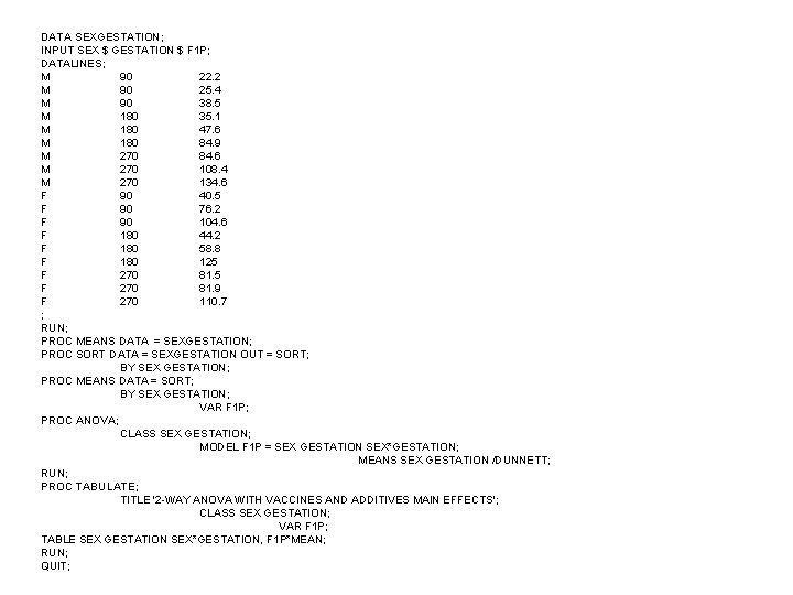
DATA SEXGESTATION; INPUT SEX $ GESTATION $ F 1 P; DATALINES; M 90 22. 2 M 90 25. 4 M 90 38. 5 M 180 35. 1 M 180 47. 6 M 180 84. 9 M 270 84. 6 M 270 108. 4 M 270 134. 6 F 90 40. 5 F 90 76. 2 F 90 104. 6 F 180 44. 2 F 180 58. 8 F 180 125 F 270 81. 9 F 270 110. 7 ; RUN; PROC MEANS DATA = SEXGESTATION; PROC SORT DATA = SEXGESTATION OUT = SORT; BY SEX GESTATION; PROC MEANS DATA = SORT; BY SEX GESTATION; VAR F 1 P; PROC ANOVA; CLASS SEX GESTATION; MODEL F 1 P = SEX GESTATION SEX*GESTATION; MEANS SEX GESTATION /DUNNETT; RUN; PROC TABULATE; TITLE '2 -WAY ANOVA WITH VACCINES AND ADDITIVES MAIN EFFECTS'; CLASS SEX GESTATION; VAR F 1 P; TABLE SEX GESTATION SEX*GESTATION, F 1 P*MEAN; RUN; QUIT;

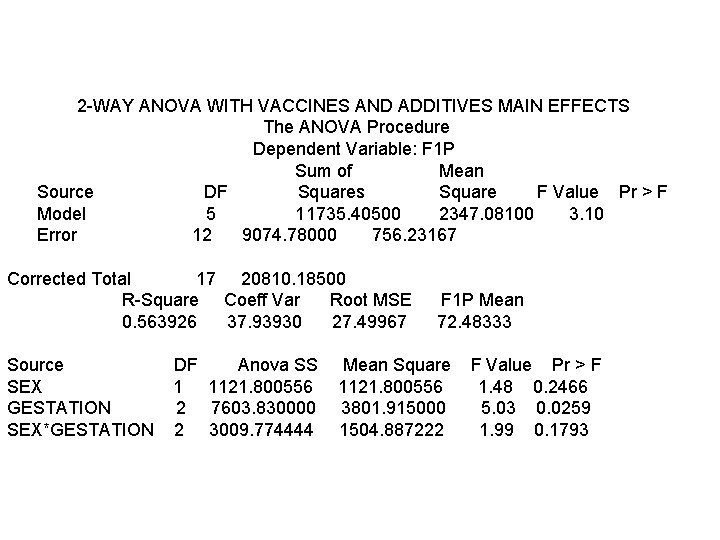
2 -WAY ANOVA WITH VACCINES AND ADDITIVES MAIN EFFECTS The ANOVA Procedure Dependent Variable: F 1 P Sum of Mean Source DF Squares Square F Value Pr > F Model 5 11735. 40500 2347. 08100 3. 10 Error 12 9074. 78000 756. 23167 Corrected Total 17 20810. 18500 R-Square Coeff Var Root MSE 0. 563926 37. 93930 27. 49967 Source SEX GESTATION SEX*GESTATION DF Anova SS 1 1121. 800556 2 7603. 830000 2 3009. 774444 F 1 P Mean 72. 48333 Mean Square 1121. 800556 3801. 915000 1504. 887222 F Value Pr > F 1. 48 0. 2466 5. 03 0. 0259 1. 99 0. 1793