ANALYSIS OF VARIANCE TECHNIQUES ANOVA ANOVA Analysis of

ANALYSIS OF VARIANCE TECHNIQUES (ANOVA)

ANOVA • Analysis of Variance (ANOVA) and t tests: are two different ways of testing for mean differences • t tests are limited to two treatment conditions • ANOVA can compare two or more treatment conditions and several DV’s • It is possible to conduct t tests between every pair of variables - increases the chances that significant findings might be one of the few due to chance (at the p =. 05 level, 1 in 20 results reach significance level by chance)

ANOVA is used when we want to know if two or more conditions or levels of the independent variable create significant mean differences on the dependent variable. The IV must be a nominal or ordinal variable identifying conditions or levels, and we compare the DV mean scores of the different levels. The DV must be a scale variable. The aim of the analysis is to identify the probability that any difference in the DV sample means for different levels of the grouping variable reflects a true difference in the population means.

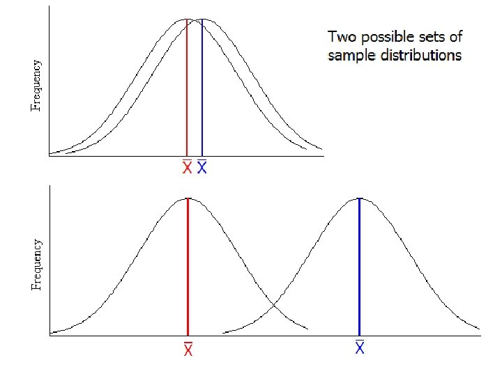
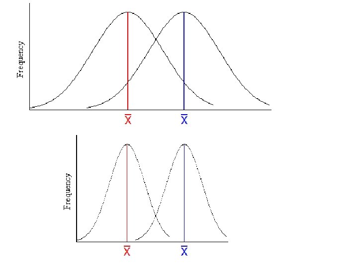
ANOVA compares two possible situations. 1. The two or more samples of the IV come from different populations of normal distributions which have similar variances (and, therefore, standard deviations) but have different population means or 2. The two or more samples come from the same population which is normally distributed. Any difference in sample means is due to sampling error. This is the default position. We should continue to believe that this is true unless we are 95% certain that it isn’t true (p <. 05).

ANOVA If we collected two samples, what would make us more certain that the two samples came from different populations? 1. The bigger the difference between two sample means, the more likely that the population means are different. 2. The smaller the variation within each group, the more likely that the population means are different.

THE LOGIC OF ANOVA • ANOVA is built on comparing variances from two sources. These two estimates are: – The Between Group variance - a measure of the effect of the independent variable plus the error variance. – The Within Groups variance - the error variance alone. • The ratio between them is called the F ratio

THE F RATIO OR STATISTIC F = Magnitude of variation between groups Magnitude of variation within groups = Between group variance Within group variance So the bigger the value for F, the larger the between group variance is to the within group variance (the random variation).

PROBABILITY – We use the F statistic to calculate the probability that the two sample means come from two different populations. – Something else is also important when calculating the probability – the larger the samples, the more likely the differences also exist in the population. – Thus the significance of F also depends on df – the larger the df the smaller the F for significance

F RATIO • A significant F ratio informs us that the group or treatment means are not all equal • When the variance between groups relative to within groups is large then the F ratio is large • The larger the F ratio the more likely it is significant and that there are significant differences between some or all group means • A small F ratio close to 1 implies that the two variance estimates are very similar

ASSUMPTIONS of ANOVA • • • Normality - ANOVA is fairly robust for departures from normality as long as they are not extreme Homogeneity of variance - This similarity of variance in each group is needed in order to ‘pool’ the variances into one Within Group source of variance Independence of errors - Error here refers to the difference between each observation or score from its own group mean. In other words each score should be independent of any other score

ANOVA FAMILY • There are many types of ANOVA just as there were statistics for measuring differences between two means. • One Way ANOVA’S are the equivalent of the Independent t test for more than two levels of the IV • Repeated Measures ANOVA’s are the equivalent of the Repeated measures t test for more than two occasions • Factorial ANOVA’s look at interactions between two or more IV’s

ONE WAY BETWEEN GROUPS ANOVA (INDEPENDENT GROUPS ANOVA) • has only one IV which splits into two or more levels • two basic variability components: – Between Groups or treatments (conditions) variability. Variability due to the differences between groups and reflected in variability between sample means. The sources of this variability are: • treatment effects, i. e. the different conditions; • individual differences, i. e. the uniqueness of people - and • experimental error, i. e. uncontrolled and unknown causes. – Within Groups or treatments (conditions) variability. There is variability within each sample as each person within a sample produced different results from others in that sample. This is due to: • individual differences; and • experimental error.

F RATIO • Once total variability is analysed into its basic components we simply compare them by computing the F ratio. • For the independent measures ANOVA : F = variability between treatments variability within treatments or between treatment variance within treatment variance Or F = treatment effect + individual differences + experimental error In the last formula the experimental error cancels out so we are testing whether the treatment effect is discernible over the expected random individual variations.

POST HOC TESTS • A Post Hoc Test is conducted after a significant F test in order to identify where significant differences lie among three or more treatments • Tukey’s HSD, Scheffe, Bonferroni and the Games-Howell procedure are commonly used. • When variances differ use the Games. Howell or Dunnett.

Example: One-Way ANOVA Test of attitude to income tax rates between three age groups (Old, Mid and Young) • • IV – AGE (three groups - nominal); DV – attitude to tax rates (score out of 10 - interval) • N = 60 • One Way ANOVA with POST HOC Analysis

Histogram of test scores by Age Groups

Results Descriptives Test score N Mean Std. Deviation 95% Confidence Interval for Between- Mean Component Std. Error Lower Bound Upper Bound Minimum Maximum Old 20 3. 7500 1. 91600 . 42843 2. 8533 4. 6467 1. 00 8. 00 Young 20 6. 3500 1. 84320 . 41215 5. 4874 7. 2126 2. 00 9. 00 Mid 20 5. 0500 2. 01246 . 45000 4. 1081 5. 9919 1. 00 8. 00 Total 60 5. 0500 2. 17400 . 28066 4. 4884 5. 6116 1. 00 9. 00 1. 92513 . 24853 4. 5523 5. 5477 . 75056 1. 8206 8. 2794 Model Fixed Effects Random Effects 211. 250 Variance 1. 5046 9

Results Test of Homogeneity of Variance Not significant so homogeneity of variances is satisfied Test Score Levene Statistic . 081 df 2 2 57 Sig. Highly significant F so significant mean differences exist . 922 ANOVA Test Score Sum of Squares Between Groups df Mean Square 67. 600 2 33. 800 Within Groups 211. 250 57 3. 706 Total 278. 850 59 F 9. 120 Sig. . 000

Interpretation Of Table • F = 9. 120 and is highly significant (p =. 000) • But are there significant differences between all the groups? • A Beronferroni Post Hoc test reveals the significant differences only lie between the young and old groups

Post Hoc Multiple Comparisons Dependent Variable: Attitude Score Bonferroni Mean 95% Confidence Interval Difference (I) Age Group (J) Age Group (I-J) Old Young -2. 6000 * . 60878 Mid -1. 3000 Old Young Mid Std. Error Lower Bound Upper Bound . 000 -4. 1017 -1. 0983 . 60878 . 111 -2. 8017 . 2017 2. 6000 * . 60878 . 000 1. 0983 4. 1017 Mid 1. 3000 . 60878 . 111 -. 2017 2. 8017 Old 1. 3000 . 60878 . 111 -. 2017 2. 8017 Young -1. 3000 . 60878 . 111 -2. 8017 . 2017 *. The mean difference is significant at the. 05 level. Sig.

INTERPRETATION OF POST HOC TEST The only significant difference on attitudes to income tax rates is between the young group and the old group (p <. 05).

REPEATED MEASURES ANALYSIS OF VARIANCE Analysis of Variance in which each individual is measured more than once so that the levels of the independent variable are the different times or types of observations for the same people

TWO FACTOR ANOVA or TWO WAY ANOVA or FACTORIAL ANOVA • When two factors of interest are to be examined at the same time • Tests a null hypothesis for each of the independent variables and also one for their interaction, the interaction effect • Interactions occur when the effect of 1 IV on the DV is not the same under all the conditions of the other IV.

FACTORIAL ANOVA Has three distinct hypotheses 1. The main effect of factor A (IV ‘A’). The null hypothesis states that there are no statistically significant mean differences between levels of factor A 2. The main effect for factor B (IV ‘B’). There is a similar null hypothesis for factor B 3. The A X B interaction. The null hypothesis states that there is no statistically significant interaction. That is the effect of either factor is independent of the levels of the other factor

Types of Interactions Age is a significant factor on performance irrespective of production method

Types of Interactions

Types of Interactions

Types of Interactions

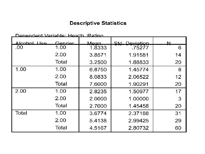
EXAMPLE OF FACTORIAL OR TWO WAY ANOVA Independent Variables: • Alcohol use (Three groups: Little or No Alcohol Use; Moderate Alcohol Use; Heavy Alcohol Use) • Gender Dependent Variable: • Self-Rated Health Status N = 60 (20 per group) Do alcohol use and gender interact in determining self health rating?

Tests of Between-Subjects Effects Dependent Variable: Health_Rating Type III Sum Source of Squares Corrected Model 314. 173 b Intercept 773. 732 Alcohol_Use 259. 470 Gender 6. 918 Alcohol_Use*Gender 13. 054 Error 150. 810 Total 1689. 000 Corrected Total 464. 983 df 5 1 2 54 60 59 Mean Square F Sig. 62. 835 22. 499. 000 773. 732 277. 048. 000 129. 735 46. 454. 000 2. 477. 121 6. 918 6. 527 2. 337. 106 2. 793 a. Computed using alpha =. 05 b. R Squared =. 676 (Adjusted R Squared =. 646) Partial Eta Observed a Squared Power. 676 1. 000. 837 1. 000. 632 1. 000. 044. 340. 080. 453

Interpretation of Previous Table • The only significant main effects F was for levels of alcohol use on self rated health (p <. 000). • There were no significant differences for either gender or the interaction between gender and alcohol use. • The following box plots and graph illustrate this

Box Plot compares self-rated health Scores for three alcohol groups

Box Plot compares self-rated health Scores for Gender

Self-Rated Health Status By Gender and Alcohol Use 10. 00 Female Male 8. 00 6. 00 4. 00 2. 00 0. 00 Little or No Alcohol Use Moderate Alcohol Use Heavy Alcohol Use

INTERPRETATION OF PAIR-WISE COMPARISONS TABLE • Since the level of alcohol consumption IV was significant it is necessary to determine whether the significance relates to all levels of alcohol consumption. • The next table reveals that significant differences (p <. 05) only lie between the moderate consumption group and the two other groups • The nil and heavy groups did not differ significantly in their self rated health status

Pairwise Comparisons Dependent Variable: Health_Rating 95% Confidence Interval Mean a for Difference a (I) Alcohol_Use (J) Alcohol_Use (I-J) Std. Error Sig. Lower Bound. Upper Bound. 00 1. 00 -4. 634 *. 558. 000 -5. 753 -3. 515 2. 00. 433. 663. 516 -. 896 1. 763 1. 00 4. 634 *. 558. 000 3. 515 5. 753 2. 00 5. 067 *. 648. 000 3. 769 6. 366 2. 00 -. 433. 663. 516 -1. 763. 896 1. 00 -5. 067 *. 648. 000 -6. 366 -3. 769 Based on estimated marginal means *. The mean difference is significant at the. 05 level. a. Adjustment for multiple comparisons: Least Significant Difference (equivalent to no adjustments).

ANALYSIS OF COVARIANCE (ANCOVA) • a form of analysis that is based on a combination of regression and ANOVA • do groups differ on a DV when you have partialled out another variable (the covariate) that has a relationship with the DV? • ANCOVA answers the question ‘What would the means of each group be on the DV if the means of the groups had the same mean on the co-variate’?

NON-PARAMETRIC ALTERNATIVES FOR ANOVA • Kruskal-Wallis One Way Non-Parametric ANOVA • Friedman Two way Non-Parametric ANOVA • Located under Non-Parametric tests in SPSS