Chapter 12 Introduction to Analysis of Variance The

Chapter 12: Introduction to Analysis of Variance

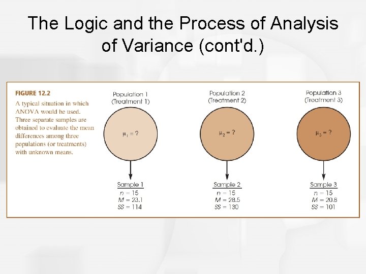
The Logic and the Process of Analysis of Variance • Chapter 12 presents the general logic and basic formulas for the hypothesis testing procedure known as analysis of variance (ANOVA). • The purpose of ANOVA is much the same as the t tests presented in the preceding chapters: the goal is to determine whether the mean differences that are obtained for sample data are sufficiently large to justify a conclusion that there are mean differences between the populations from which the samples were obtained.

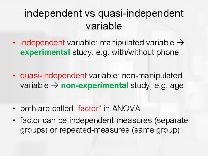
independent vs quasi-independent variable • independent variable: manipulated variable experimental study, e. g. with/without phone • quasi-independent variable: non-manipulated variable non-experimental study, e. g. age • both are called “factor” in ANOVA • factor can be independent-measures (separate groups) or repeated-measures (same group)

ch 12 - ch 14 • ch 12: 1 -factor independent-measures designs • ch 13: 1 -factor repeated-measures designs • ch 14: 2 -factor designs (factorial designs)

The Logic and the Process of Analysis of Variance (cont'd. ) • The difference between ANOVA and the t tests is that ANOVA can be used in situations where there are two or more means being compared, whereas the t tests are limited to situations where only two means are involved. • ANOVA is necessary to protect researchers from excessive risk of a Type I error in situations where a study is comparing more than two population means.

The Logic and the Process of Analysis of Variance (cont'd. ) • These situations would require a series of several t tests to evaluate all of the mean differences. (Remember, a t test can compare only two means at a time. ) • Although each t test can be done with a specific α-level (risk of Type I error), the α-levels accumulate over a series of tests so that the final experimentwise α-level can be quite large.

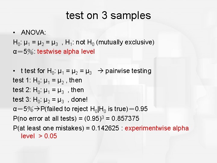
test on 3 samples • ANOVA: H 0: μ 1 = μ 2 = μ 3 , H 1: not H 0 (mutually exclusive) α＝ 5％: testwise alpha level • t test for H 0: μ 1 = μ 2 = μ 3 pairwise testing test 1: H 0: μ 1 = μ 2 , then test 2: H 0: μ 1 = μ 3 , then test 3: H 0: μ 2 = μ 3 , done! α＝ 5％ P(failed to reject H 0|H 0 is true)＝ 0. 95 P(no error at all tests) = (0. 95)3 = 0. 857375 P(at least one mistakes) = 0. 142625 : experimentwise alpha level > 0. 05

The Logic and the Process of Analysis of Variance (cont'd. ) • ANOVA allows researcher to evaluate all of the mean differences in a single hypothesis test using a single α-level and, thereby, keeps the risk of a Type I error under control no matter how many different means are being compared. • Although ANOVA can be used in a variety of different research situations, this chapter presents only independent-measures designs involving only one independent variable. • i. e. 1 -factor independent-measures designs

The Logic and the Process of Analysis of Variance (cont'd. )

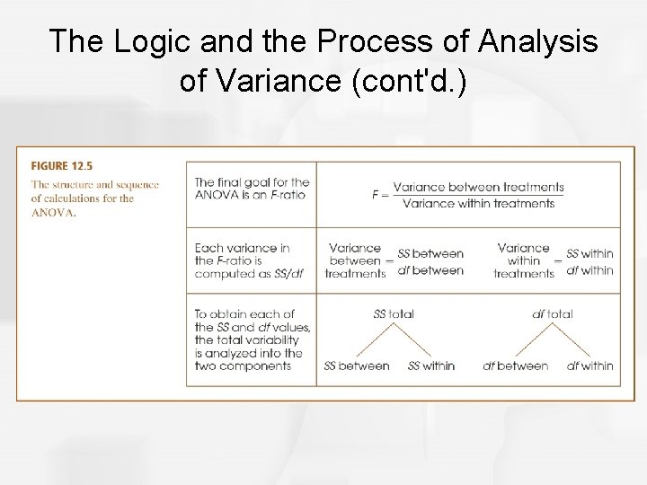
The Logic and the Process of Analysis of Variance (cont'd. ) • The test statistic for ANOVA is an F-ratio, which is a ratio of two sample variances. In the context of ANOVA, the sample variances are called mean squares, or MS values. • The top of the F-ratio, MSbetween, measures the size of mean differences between samples. The bottom of the ratio, MSwithin, measures the magnitude of differences that would be expected without any treatment effects.

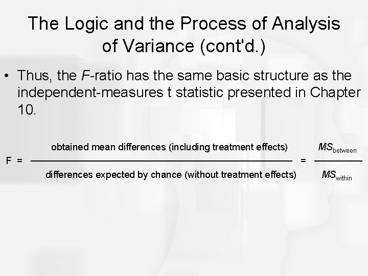
The Logic and the Process of Analysis of Variance (cont'd. ) • Thus, the F-ratio has the same basic structure as the independent-measures t statistic presented in Chapter 10. obtained mean differences (including treatment effects) MSbetween F = ─────────────────── = ─────── differences expected by chance (without treatment effects) MSwithin

The Logic and the Process of Analysis of Variance (cont'd. )

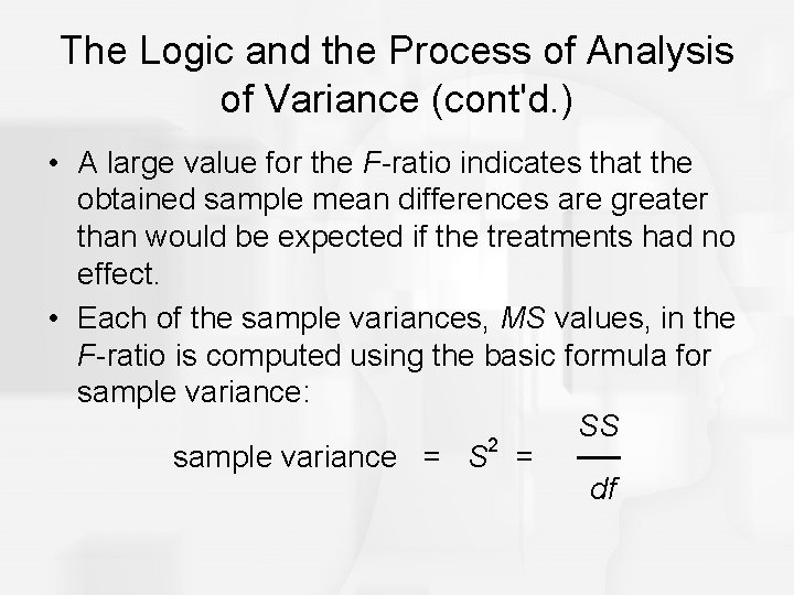
The Logic and the Process of Analysis of Variance (cont'd. ) • A large value for the F-ratio indicates that the obtained sample mean differences are greater than would be expected if the treatments had no effect. • Each of the sample variances, MS values, in the F-ratio is computed using the basic formula for sample variance: SS 2 sample variance = S = ── df

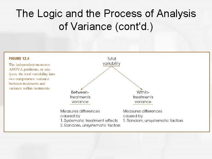
The Logic and the Process of Analysis of Variance (cont'd. ) • To obtain the SS and df values, you must go through an analysis that separates the total variability for the entire set of data into two basic components: within-treatment variability (which will be the denominator: MSE) and betweentreatment variability (which will become the numerator of the F-ratio: MST).

The Logic and the Process of Analysis of Variance (cont'd. ) • The two components of the F-ratio can be described as follows: • Within-Treatments Variability: MSwithin measures the size of the differences that exist inside each of the samples. (MSE) • Because all the individuals in a sample receive exactly the same treatment, any differences (or variance) within a sample cannot be caused by different treatments.

The Logic and the Process of Analysis of Variance (cont'd. ) • Thus, these differences are caused by only one source: (MSE) – Chance or Error: The unpredictable differences that exist between individual scores are not caused by any systematic factors and are simply considered to be random chance or error.

The Logic and the Process of Analysis of Variance (cont'd. ) • Between-Treatments Variability: MSbetween measures the size of the differences between the sample means. For example, suppose that three treatments, each with a sample of n = 5 subjects, have means of M 1 = 1, M 2 = 2, and M 3 = 3. (MST) • Notice that the three means are different; that is, they are variable.

The Logic and the Process of Analysis of Variance (cont'd. ) • By computing the variance for the three means we can measure the size of the differences. • Although it is possible to compute a variance for the set of sample means, it usually is easier to use the total, T, for each sample instead of the mean, and compute variance for the set of T values.

The Logic and the Process of Analysis of Variance (cont'd. ) • Logically, the differences (or variance) between means can be caused by two sources: – Treatment Effects: If the treatments have different effects, this could cause the mean for one treatment to be higher (or lower) than the mean for another treatment. – Chance or Sampling Error: If there is no treatment effect at all, you would still expect some differences between samples. Mean differences from one sample to another are an example of random, unsystematic sampling error.

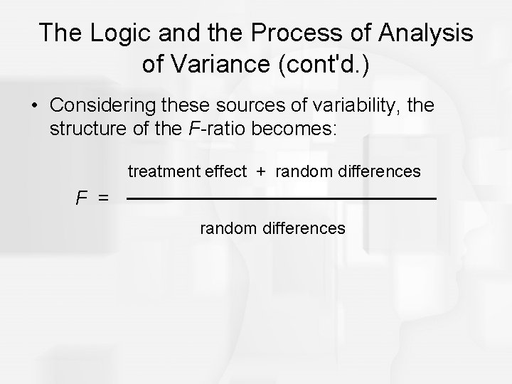
The Logic and the Process of Analysis of Variance (cont'd. ) • Considering these sources of variability, the structure of the F-ratio becomes: treatment effect + random differences F = ─────────── random differences

The Logic and the Process of Analysis of Variance (cont'd. ) • When the null hypothesis is true and there are no differences between treatments, the F-ratio is balanced. • That is, when the "treatment effect" is zero, the top and bottom of the F-ratio are measuring the same variance. • In this case, you should expect an F-ratio near 1. 00. When the sample data produce an F-ratio near 1. 00, we will conclude that there is no significant treatment effect.

The Logic and the Process of Analysis of Variance (cont'd. ) • On the other hand, a large treatment effect will produce a large value for the F-ratio. Thus, when the sample data produce a large F-ratio we will reject the null hypothesis and conclude that there are significant differences between treatments. • To determine whether an F-ratio is large enough to be significant, you must select an α-level, find the df values for the numerator and denominator of the F-ratio, and consult the F-distribution table to find the critical value.

The Logic and the Process of Analysis of Variance (cont'd. )

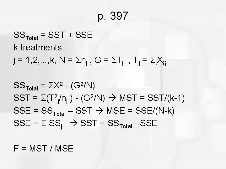
p. 397 SSTotal = SST + SSE k treatments: j = 1, 2, . . . , k, N = Σnj , G = ΣTj , Tj = Σi. Xij SSTotal = ΣX 2 - (G 2/N) SST = Σ(T 2 j/nj ) - (G 2/N) MST = SST/(k-1) SSE = SSTotal – SST MSE = SSE/(N-k) SSE = Σ SSj SST = SSTotal - SSE F = MST / MSE

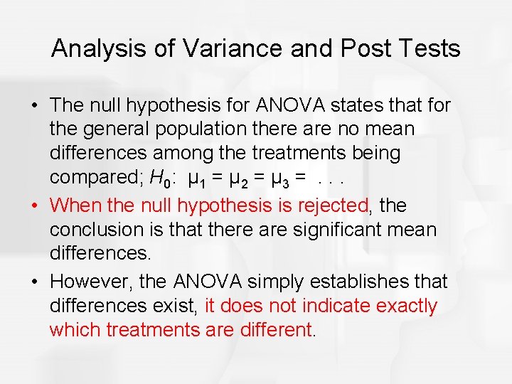
Analysis of Variance and Post Tests • The null hypothesis for ANOVA states that for the general population there are no mean differences among the treatments being compared; H 0: μ 1 = μ 2 = μ 3 =. . . • When the null hypothesis is rejected, the conclusion is that there are significant mean differences. • However, the ANOVA simply establishes that differences exist, it does not indicate exactly which treatments are different.

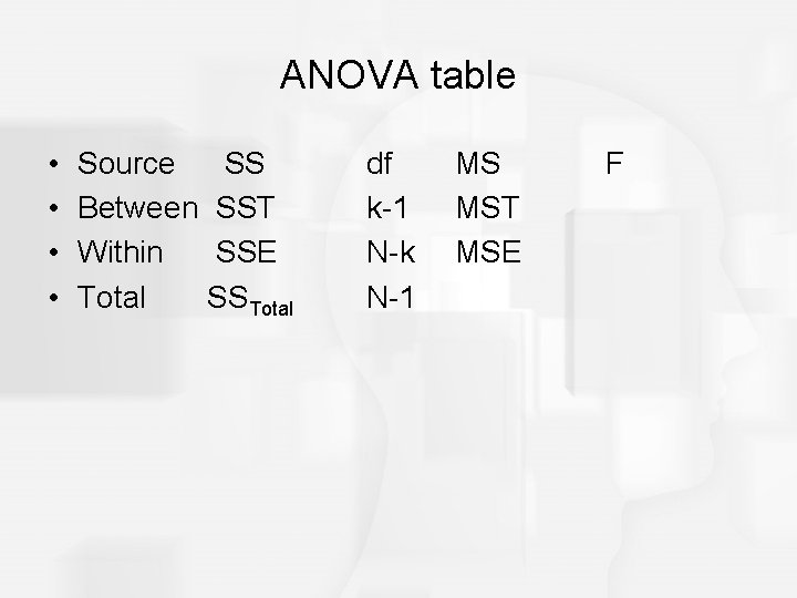
ANOVA table • • Source SS Between SST Within SSE Total SSTotal df k-1 N-k N-1 MS MST MSE F

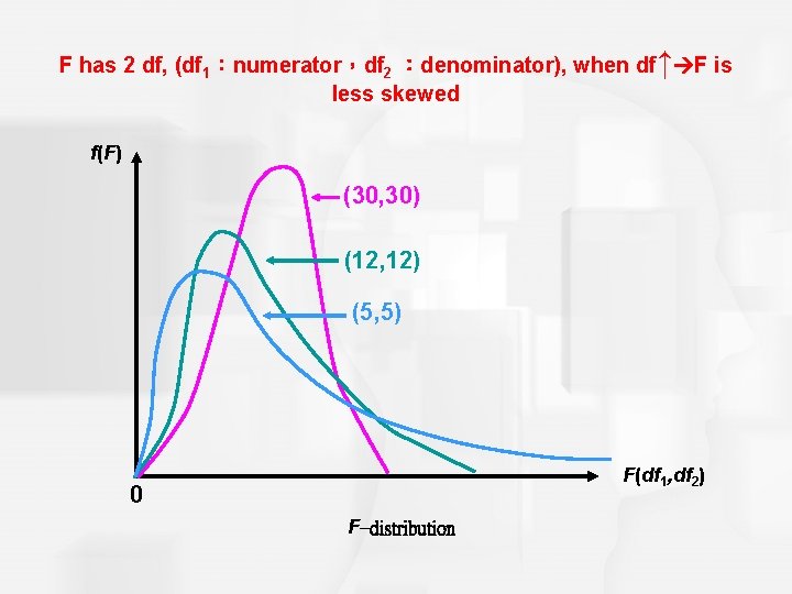
LO 12 -1 Characteristics of a F-Distribution § There is a “family” of F- distributions. A particular member of the family is determined by two parameters: the degrees of freedom in the numerator and the degrees of freedom in the denominator. § The F-distribution is continuous. § A F-value cannot be negative i. e. ： F>0. § The F-distribution is positively skewed. § It is asymptotic. As F , the curve approaches the X-axis but never touches it. 12 -*

F has 2 df, (df 1：numerator，df 2 ：denominator), when df↑ F is less skewed f(F) (30, 30) (12, 12) (5, 5) F(df 1, df 2) 0 F–distribution

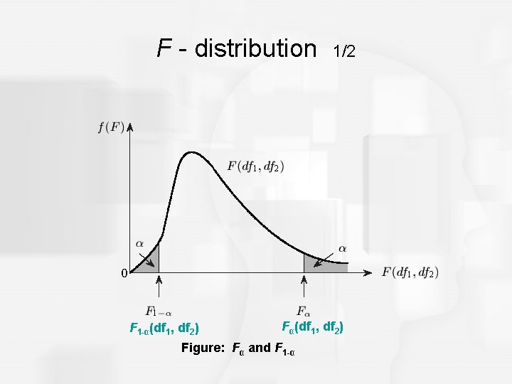
F - distribution F 1 -α(df 1, df 2) 1/2 Fα(df 1, df 2) Figure: Fα and F 1 -α

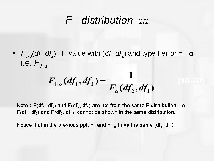
F - distribution 2/2 • F 1 -α(df 1, df 2) : F-value with (df 1, df 2) and type I error =1 -α , i. e. F 1 -α : (10 -30) Note：F(df 1, df 2) and F(df 2, df 1) are not from the same F distribution, i. e. F(df 1, df 2) and F(df 2, df 1) cannot be shown in the same distribution. Notice that in the previous ppt: Fα and F 1 -α have the same (df 1, df 2)

Measuring Effect Size for an Analysis of Variance • As with other hypothesis tests, an ANOVA evaluates the significance of the sample mean differences; that is, are the differences bigger than would be reasonable to expect just by chance. • With large samples, however, it is possible for relatively small mean differences to be statistically significant. • Thus, the hypothesis test does not necessarily provide information about the actual size of the mean differences.

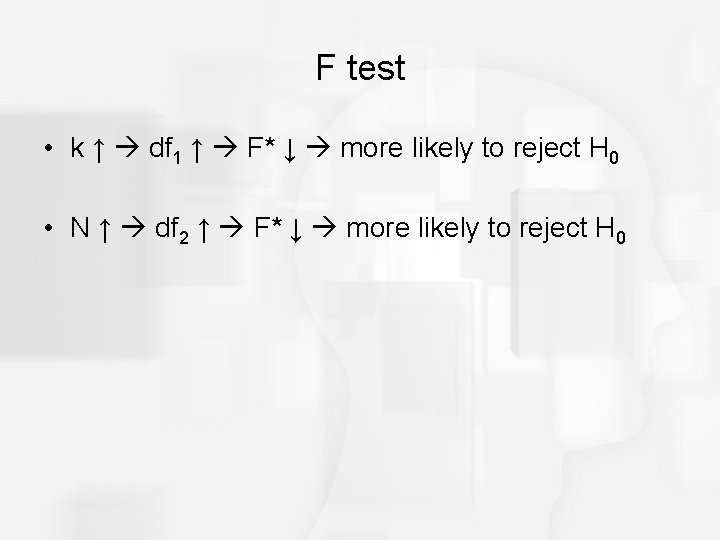
F test • k ↑ df 1 ↑ F* ↓ more likely to reject H 0 • N ↑ df 2 ↑ F* ↓ more likely to reject H 0

Measuring Effect Size for an Analysis of Variance (cont'd. ) • To supplement the hypothesis test, it is recommended that you calculate a measure of effect size. • For an analysis of variance the common technique for measuring effect size is to compute the percentage of variance that is accounted for by the treatment effects.

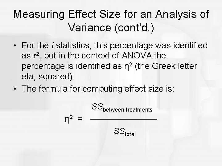
Measuring Effect Size for an Analysis of Variance (cont'd. ) • For the t statistics, this percentage was identified as r 2, but in the context of ANOVA the percentage is identified as η 2 (the Greek letter eta, squared). • The formula for computing effect size is: SSbetween treatments η 2 = ────── SStotal

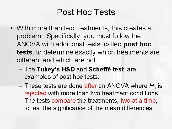
Post Hoc Tests • With more than two treatments, this creates a problem. Specifically, you must follow the ANOVA with additional tests, called post hoc tests, to determine exactly which treatments are different and which are not. – The Tukey’s HSD and Scheffé test are examples of post hoc tests. – These tests are done after an ANOVA where H 0 is rejected with more than two treatment conditions. The tests compare the treatments, two at a time, to test the significance of the mean differences.