ANALYSIS OF VARIANCE ANalysis Of Variance Lecture 16

- Slides: 38

ANALYSIS OF VARIANCE ANalysis Of Variance Lecture - 16 3/6/2021 2: 31 AM 1

• Two-sample t-test compares the difference between means in two groups • To analyse and interpret observations of several groups, we use Analysis of Variance • The different groups may be receiving different treatments, conditions, etc. • Like in two-sample comparison , we would like to compare the different treatment /group means in the population. • This method was developed by Sir Ronald A. Fisher. 3/6/2021 2: 31 AM 2

• Definition: • Analysis of Variance is a technique whereby the total variation present in a set of data is partitioned into two or more components. Associated with each of these components is a specific source of variation, so that in the analysis it is possible to ascertain the magnitude of the contributions of these sources to the total variation. 3/6/2021 2: 31 AM 3

• ANOVA has wide applications in the analysis of data derived from experiments. • Two different purposes of ANOVA are: – To estimate and test hypotheses about population variances – To estimate and test hypotheses about population means ( this is the major focus in our study ) 3/6/2021 2: 31 AM 4

An example • We wish to know whether three drugs are equally effective in lowering serum cholesterol in human subjects. Consider three independent groups of subjects and treat them with the three drugs. Measure the change in the serum cholesterol level after a specified period of time. • The change may not be at the same level in the three groups- there is variability between groups • There can be variability within group due to differences in the genetic makeup of the subjects or differences in diets. 3/6/2021 2: 31 AM 5

• Our focus is on the response variable( change in cholesterol level) to treatments ( drug used • Here the question to be answered is : Do the different values of the treatment variable result in differences, on the average, in the response variable? 3/6/2021 2: 31 AM 6

Assumptions • Analysis of variance is considered in the analysis of data from different experimental designs. The most common assumptions are of homogenity of variances and the normality of the population from which the data is sampled. • Additional assumptions depend on the experimental design used. 3/6/2021 2: 31 AM 7

ANOVA Procedure • Description of data- tabular format based on the design • Assumptions -include those of the model • Hypotheses- null and alternative; testing for the equality of population means in the different groups • Test statistic – decided based on the hypothesis • Distribution of test statistic ( results in F-statistic) 3/6/2021 2: 31 AM 8

• Decision rule – specifies the conditions for rejecting or not rejecting the null hypothesis • Calculation of test statistic , critical value/pvalue • Statistical decision – test is significant/not significant • Conclusion- translating the statistical decision into the researchers conclusion 3/6/2021 2: 31 AM 9

One-way ANOVA • Suppose we compare several groups( say five groups ) for difference in population means. If we make pairwise comparisons, then we have to make ten comparisons using two-sample ttest ten times. • This is a tedious procedure and likely to lead to false conclusions. Also the type-I error will increase • ANOVA is the solution in this case. 3/6/2021 2: 31 AM 10

• One-way ANOVA is the simplest type of ANOVA, in which only one type of variation ( one factor ) is investigated. This can be viewed as an extension of two-sample t-test ( or a particular case of One-way ANOVA. • In a typical setting of one-way ANOVA, we test the null hypothesis that three or more treatments are equally effective. 3/6/2021 2: 31 AM 11

• The experimental design needed to test this hypothesis is the completely randomised design • Here the treatments are assigned to the subjects at random • Suppose there are 16 subjects to whom four different drugs are to be allotted. A random allocation may give the following design 3/6/2021 2: 31 AM 12

Drug A: 16, 9, 15, 6 (Sl. no. of subjects) Drug. B : 14, 11, 2, 4 Drug C: 10, 7, 5, 13 Drug D: 3, 12, 1, 8 In general, for k- treatment groups, the data can be organised in the form of an array. • Note: It is possible that no. of subjects in each group may be different. • • • 3/6/2021 2: 31 AM 13

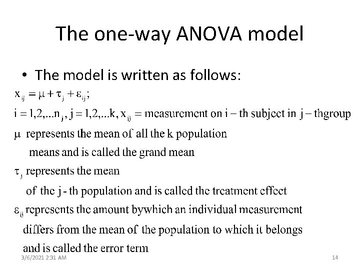
The one-way ANOVA model • The model is written as follows: 3/6/2021 2: 31 AM 14

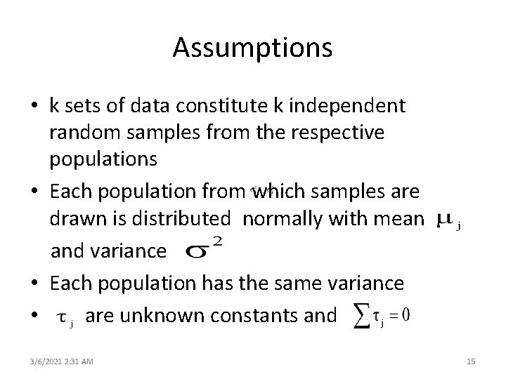
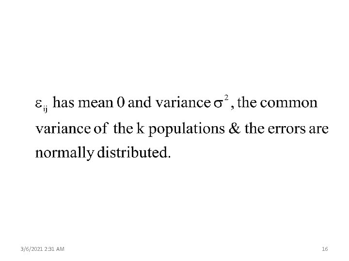
Assumptions • k sets of data constitute k independent random samples from the respective populations • Each population from which samples are drawn is distributed normally with mean and variance • Each population has the same variance • are unknown constants and 3/6/2021 2: 31 AM 15

3/6/2021 2: 31 AM 16

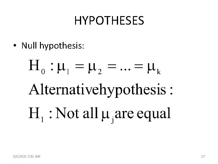
HYPOTHESES • Null hypothesis: 3/6/2021 2: 31 AM 17

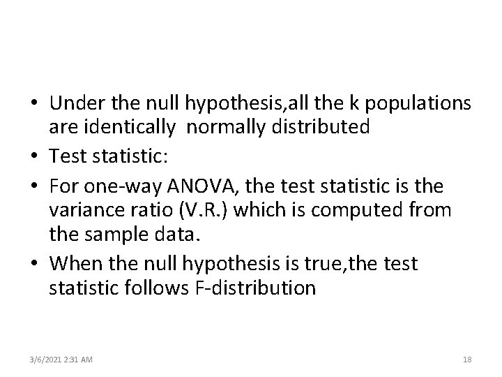
• Under the null hypothesis, all the k populations are identically normally distributed • Test statistic: • For one-way ANOVA, the test statistic is the variance ratio (V. R. ) which is computed from the sample data. • When the null hypothesis is true, the test statistic follows F-distribution 3/6/2021 2: 31 AM 18

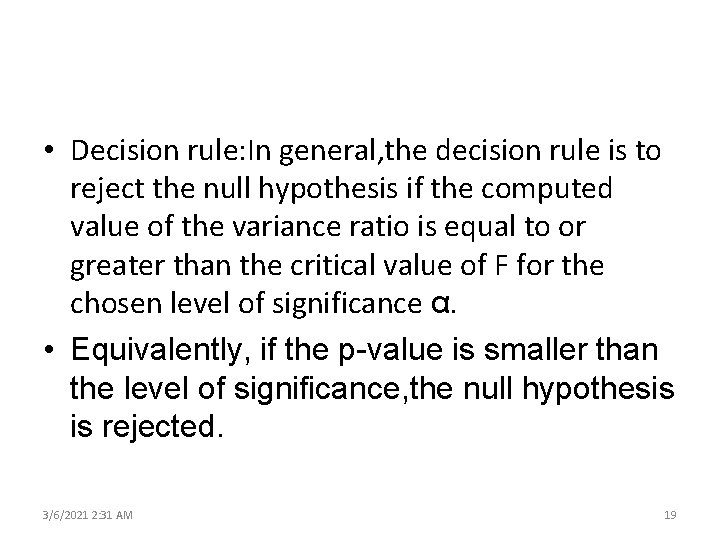
• Decision rule: In general, the decision rule is to reject the null hypothesis if the computed value of the variance ratio is equal to or greater than the critical value of F for the chosen level of significance α. • Equivalently, if the p-value is smaller than the level of significance, the null hypothesis is rejected. 3/6/2021 2: 31 AM 19

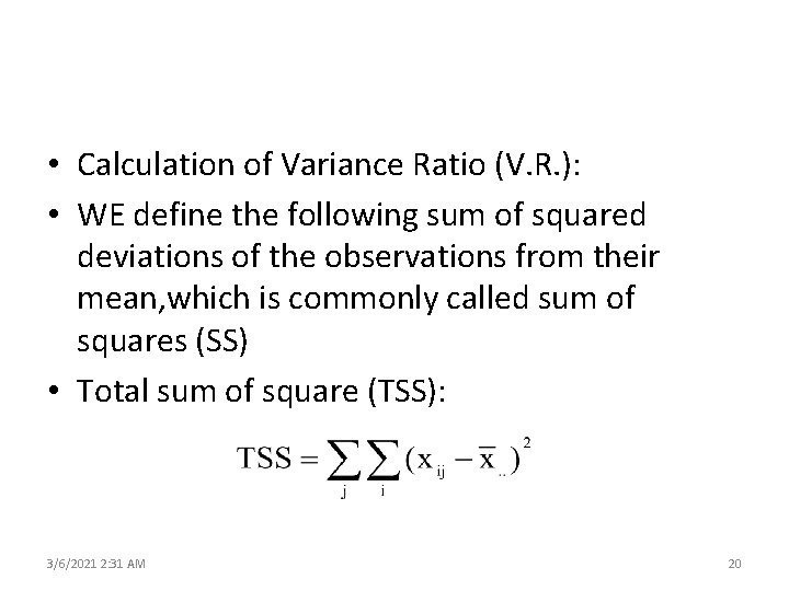
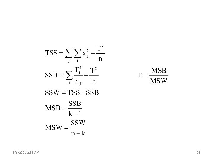
• Calculation of Variance Ratio (V. R. ): • WE define the following sum of squared deviations of the observations from their mean, which is commonly called sum of squares (SS) • Total sum of square (TSS): 3/6/2021 2: 31 AM 20

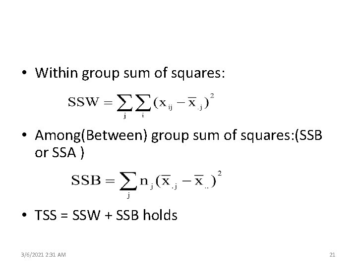
• Within group sum of squares: • Among(Between) group sum of squares: (SSB or SSA ) • TSS = SSW + SSB holds 3/6/2021 2: 31 AM 21

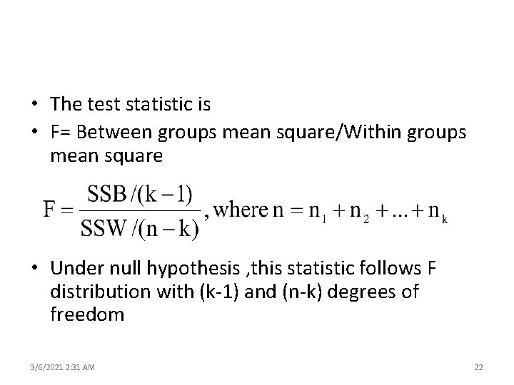
• The test statistic is • F= Between groups mean square/Within groups mean square • Under null hypothesis , this statistic follows F distribution with (k-1) and (n-k) degrees of freedom 3/6/2021 2: 31 AM 22

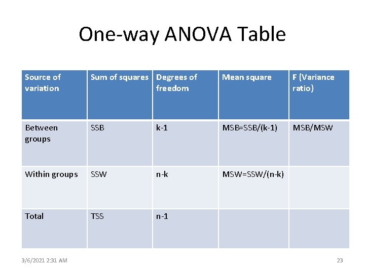
One-way ANOVA Table Source of variation Sum of squares Degrees of freedom Mean square F (Variance ratio) Between groups SSB k-1 MSB=SSB/(k-1) MSB/MSW Within groups SSW n-k MSW=SSW/(n-k) Total TSS n-1 3/6/2021 2: 31 AM 23

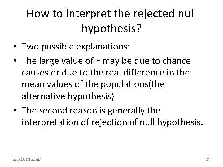
How to interpret the rejected null hypothesis? • Two possible explanations: • The large value of F may be due to chance causes or due to the real difference in the mean values of the populations(the alternative hypothesis) • The second reason is generally the interpretation of rejection of null hypothesis. 3/6/2021 2: 31 AM 24

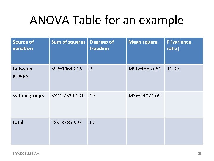
ANOVA Table for an example Source of variation Sum of squares Degrees of freedom Mean square F (variance ratio) Between groups SSB=14649. 15 3 MSB=4883. 051 11. 99 Within groups SSW=23210. 91 57 MSW=407. 209 total TSS=37860. 07 60 3/6/2021 2: 31 AM 25

• Statistical decision: The calculated value of Fstatistic is greater than the critical value (=3. 36). Hence we reject the null hypothesis. The p-value is <0. 05 ( p-value=3. 42 E 06). Hence the test is significant. • Conclusion: There is significant difference in the mean weights of animals in the four groups(populations) 3/6/2021 2: 31 AM 26

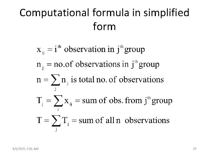
Computational formula in simplified form 3/6/2021 2: 31 AM 27

3/6/2021 2: 31 AM 28

• Rejecting the null hypothesis in ANOVA implies that there is significant difference in the mean values of the groups. Which pair/s of group means differ significantly? • To answer this question , we perform post-hoc analysis ( multiple comparison tests ) 3/6/2021 2: 32 AM 29

Post Hoc Testing • Post Hoc testing • used to determine which mean or group of means is/are significantly different from the others • many different choices depending upon research design and research question are available (Bonferroni, Duncan’s, Scheffé’s, Dunnet’s, Tukey’s HSD, . . . ) • only done when ANOVA yields a significant F 3/6/2021 2: 32 AM 30

Scheffé test: • when sample sizes are unequal • when most conservative test is desired • Critical value: Use critical value from ANOVA and • multiply by ( k-1). k = number of groups (means) • F'critical = (k– 1) Fcritical 3/6/2021 2: 32 AM 31

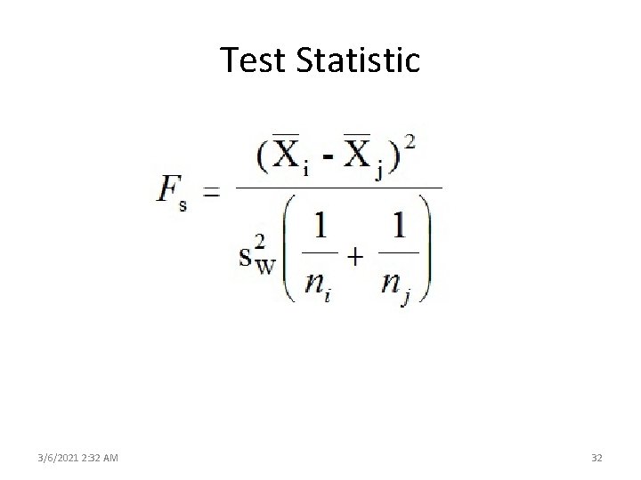
Test Statistic 3/6/2021 2: 32 AM 32

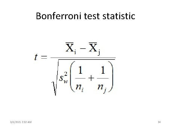
• If Fs > F'critical, then the two means are significantly different. • Bonferroni test: used when less conservative test is desirable, i. e. , more powerful • may be used with other types of statistical tests (e. g. , multiple t-tests) • when only some pairs of sample means are to be tested 3/6/2021 2: 32 AM 33

Bonferroni test statistic 3/6/2021 2: 32 AM 34

• Critical value: • Adjust α by dividing by number of all possible pairings. • Decision: • If t > t critical, then the means are significantly • different. 3/6/2021 2: 32 AM 35

Tukey HSD test (Honestly Significant Difference) • sample sizes can be equal or unequal. • used when less conservative test is desirable, i. e. , more powerful • when all pairs of sample means are to be tested • This test makes use of a single value against which all differences are compared. 3/6/2021 2: 32 AM 36

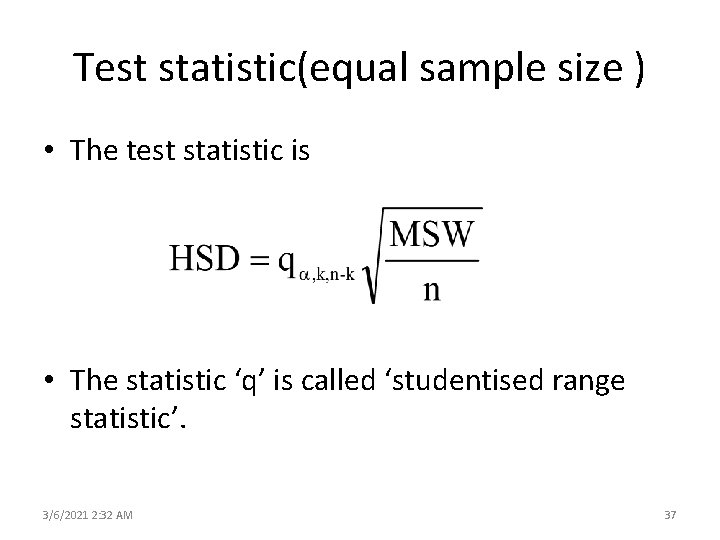
Test statistic(equal sample size ) • The test statistic is • The statistic ‘q’ is called ‘studentised range statistic’. 3/6/2021 2: 32 AM 37

• It is defined as the difference between the largest and smallest treatment means from an ANOVA. • All possible differences between pairs of means are computed, and any difference that gives an absolute value that exceeds HSD is declared to be significant. • When sample sizes are unequal, compute HSD by replacing ‘n’ by , which is the smallest of the two sample sizes that are to be compared. 3/6/2021 2: 32 AM 38