The Analysis of Variance The Analysis of Variance



- Slides: 23

The Analysis of Variance

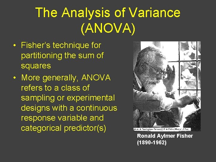
The Analysis of Variance (ANOVA) • Fisher’s technique for partitioning the sum of squares • More generally, ANOVA refers to a class of sampling or experimental designs with a continuous response variable and categorical predictor(s) Ronald Aylmer Fisher (1890 -1962)

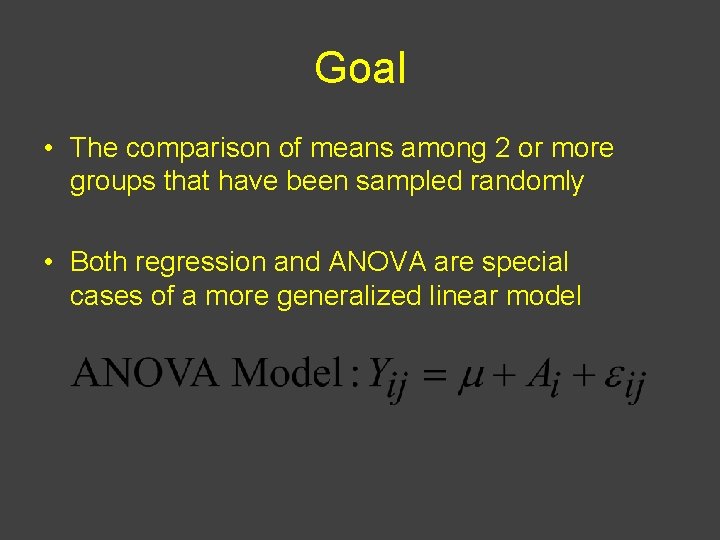
Goal • The comparison of means among 2 or more groups that have been sampled randomly • Both regression and ANOVA are special cases of a more generalized linear model

ANOVA & Partitioning the Sum of Squares 1. Remember: total variation is the sum of the difference between each observation and the overall sample mean 2. Using ANOVA, we can partition the sum of squares among the different components in the model (the treatments, the error term, etc. ) 3. Finally, we can use the results to test statistical hypotheses about the strength of particular effects

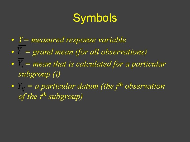
Symbols • Y= measured response variable • = grand mean (for all observations) • = mean that is calculated for a particular subgroup (i) • = a particular datum (the jth observation of the ith subgroup)

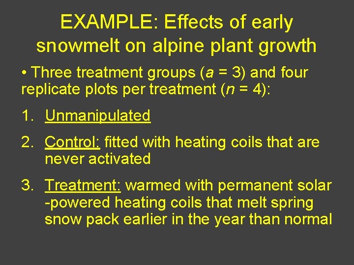
EXAMPLE: Effects of early snowmelt on alpine plant growth • Three treatment groups (a = 3) and four replicate plots per treatment (n = 4): 1. Unmanipulated 2. Control: fitted with heating coils that are never activated 3. Treatment: warmed with permanent solar -powered heating coils that melt spring snow pack earlier in the year than normal

Effects of early snowmelt on alpine plant growth • After 3 years of treatment application, you measure the length of the flowering period, in weeks, for larkspur (Delphinium nuttallianum) in each plot

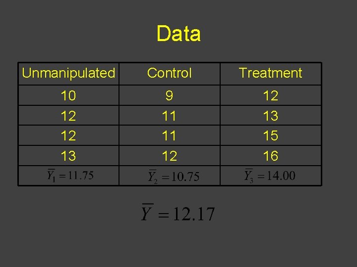
Data Unmanipulated Control Treatment 10 12 12 13 9 11 11 12 12 13 15 16

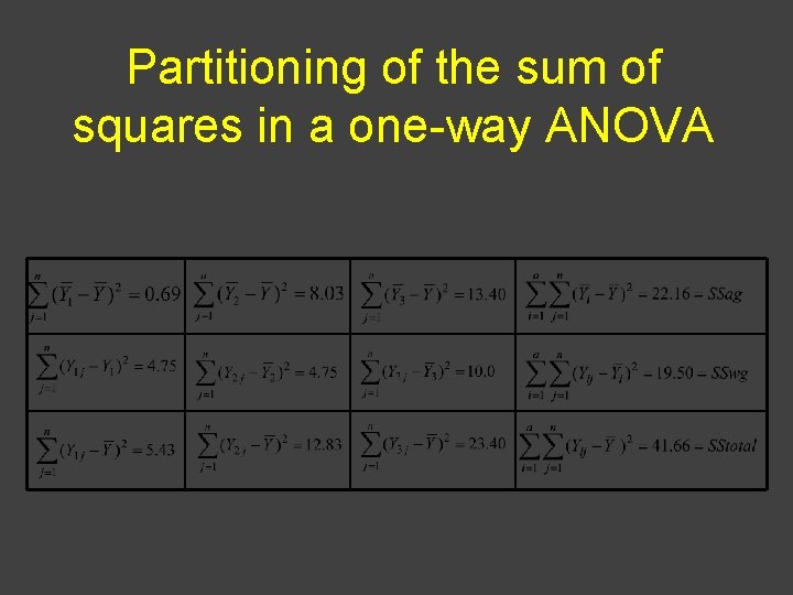
Partitioning of the sum of squares in a one-way ANOVA

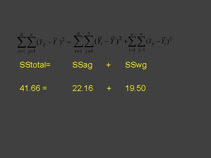
SStotal= SSag + SSwg 41. 66 = 22. 16 + 19. 50

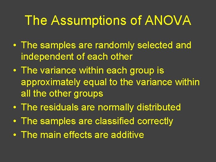
The Assumptions of ANOVA • The samples are randomly selected and independent of each other • The variance within each group is approximately equal to the variance within all the other groups • The residuals are normally distributed • The samples are classified correctly • The main effects are additive

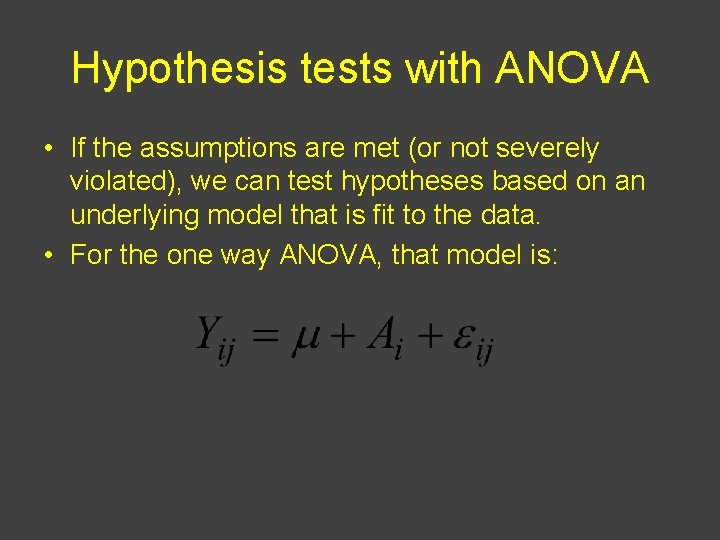
Hypothesis tests with ANOVA • If the assumptions are met (or not severely violated), we can test hypotheses based on an underlying model that is fit to the data. • For the one way ANOVA, that model is:

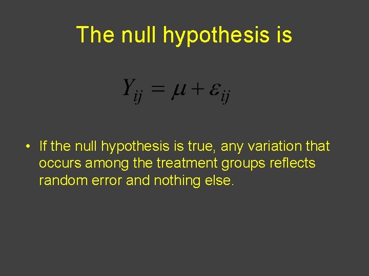
The null hypothesis is • If the null hypothesis is true, any variation that occurs among the treatment groups reflects random error and nothing else.

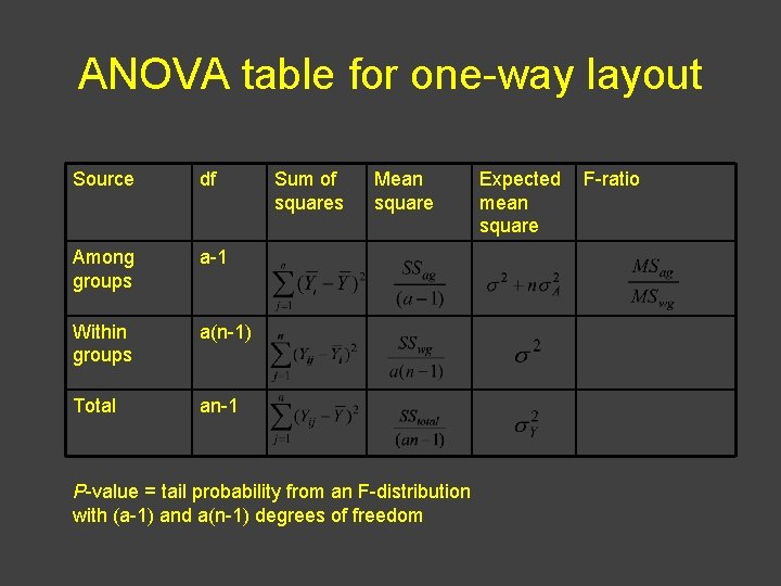
ANOVA table for one-way layout Source df Among groups a-1 Within groups a(n-1) Total an-1 Sum of squares Mean square P-value = tail probability from an F-distribution with (a-1) and a(n-1) degrees of freedom Expected mean square F-ratio

Partitioning of the sum of squares in a one-way ANOVA

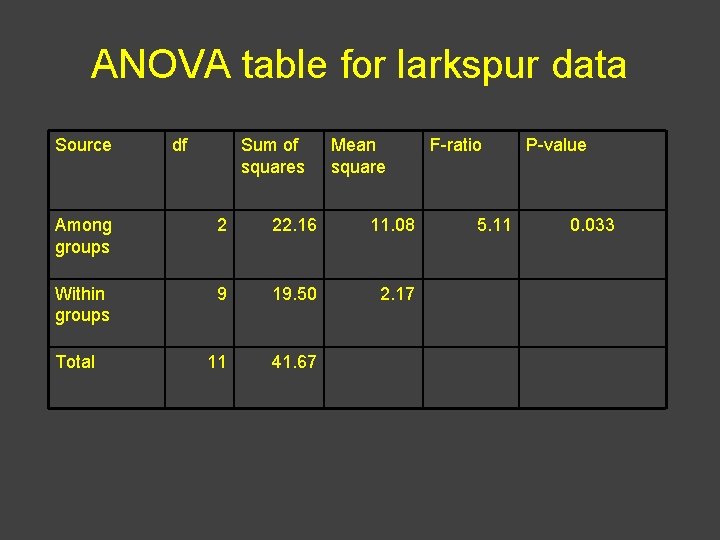
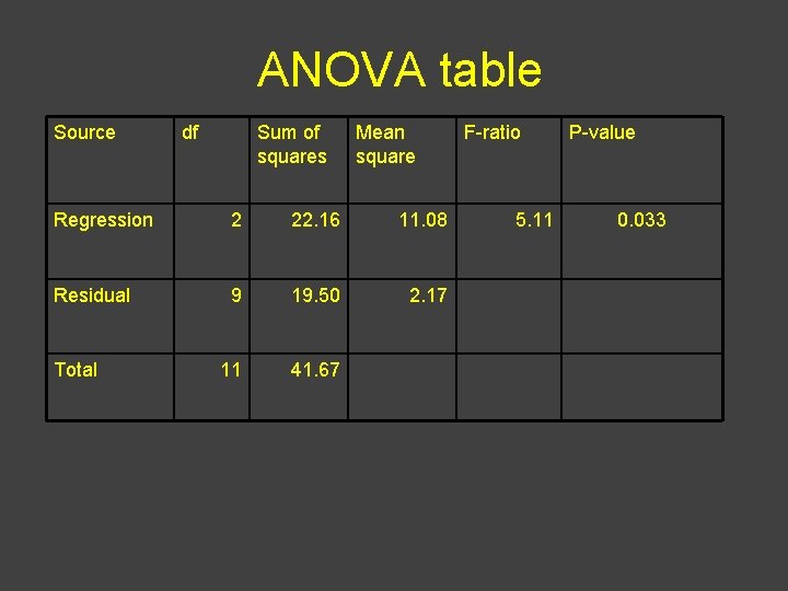
ANOVA table for larkspur data Source df Sum of squares Mean square Among groups 2 22. 16 11. 08 Within groups 9 19. 50 2. 17 11 41. 67 Total F-ratio 5. 11 P-value 0. 033

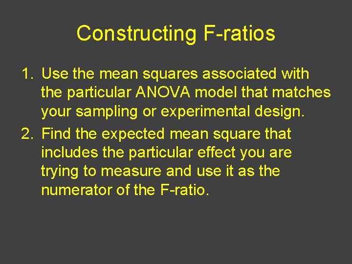
Constructing F-ratios 1. Use the mean squares associated with the particular ANOVA model that matches your sampling or experimental design. 2. Find the expected mean square that includes the particular effect you are trying to measure and use it as the numerator of the F-ratio.

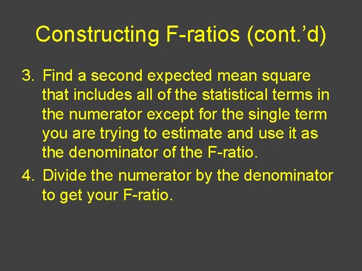
Constructing F-ratios (cont. ’d) 3. Find a second expected mean square that includes all of the statistical terms in the numerator except for the single term you are trying to estimate and use it as the denominator of the F-ratio. 4. Divide the numerator by the denominator to get your F-ratio.

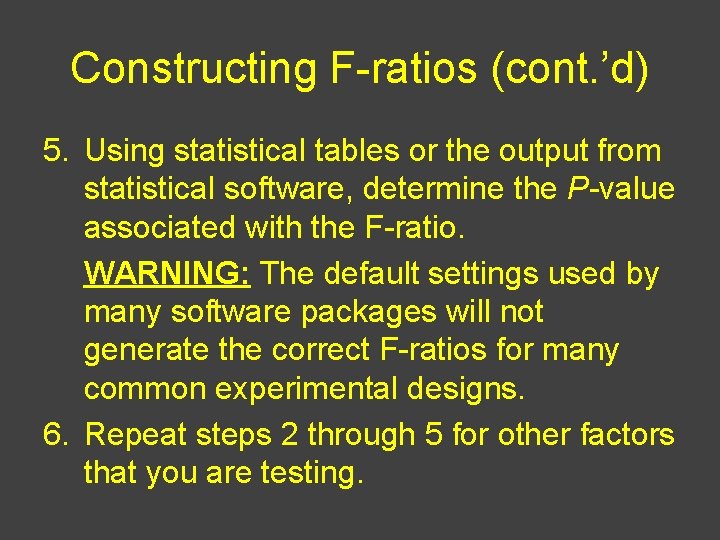
Constructing F-ratios (cont. ’d) 5. Using statistical tables or the output from statistical software, determine the P-value associated with the F-ratio. WARNING: The default settings used by many software packages will not generate the correct F-ratios for many common experimental designs. 6. Repeat steps 2 through 5 for other factors that you are testing.

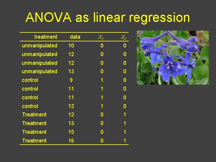
ANOVA as linear regression treatment data X 1 X 2 unmanipulated 10 0 0 unmanipulated 12 0 0 unmanipulated 13 0 0 control 9 1 0 control 11 1 0 control 12 1 0 Treatment 12 0 1 Treatment 13 0 1 Treatment 15 0 1 Treatment 16 0 1

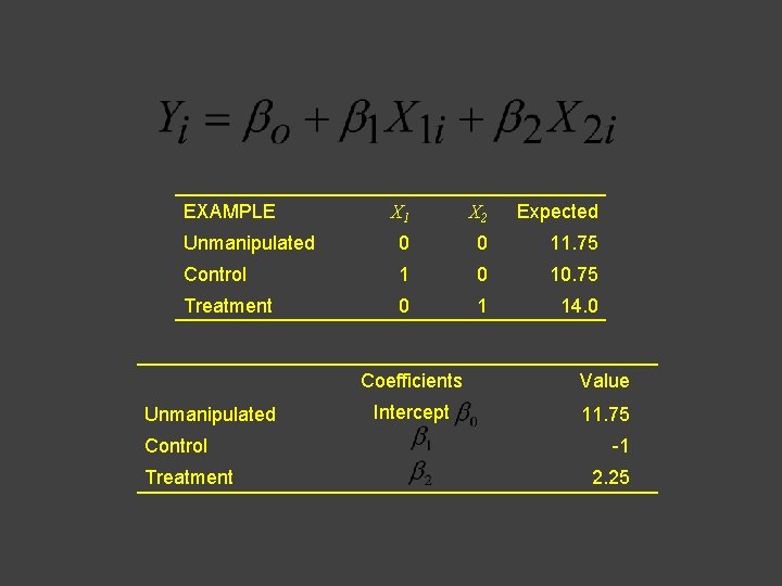
EXAMPLE X 1 X 2 Expected Unmanipulated 0 0 11. 75 Control 1 0 10. 75 Treatment 0 1 14. 0 Unmanipulated Control Treatment Coefficients Value Intercept 11. 75 -1 2. 25

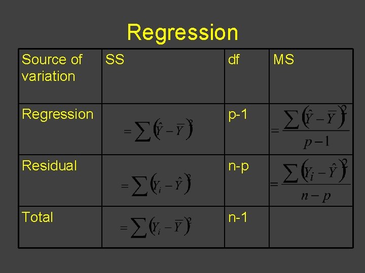
Regression Source of variation SS df Regression p-1 Residual n-p Total n-1 MS

ANOVA table Source df Sum of squares Mean square Regression 2 22. 16 11. 08 Residual 9 19. 50 2. 17 11 41. 67 Total F-ratio 5. 11 P-value 0. 033