Analysis of Variance ANOVA q A singlefactor ANOVA

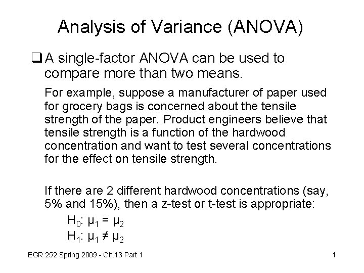
Analysis of Variance (ANOVA) q A single-factor ANOVA can be used to compare more than two means. For example, suppose a manufacturer of paper used for grocery bags is concerned about the tensile strength of the paper. Product engineers believe that tensile strength is a function of the hardwood concentration and want to test several concentrations for the effect on tensile strength. If there are 2 different hardwood concentrations (say, 5% and 15%), then a z-test or t-test is appropriate: H 0: μ 1 = μ 2 H 1: μ 1 ≠ μ 2 EGR 252 Spring 2009 - Ch. 13 Part 1 1

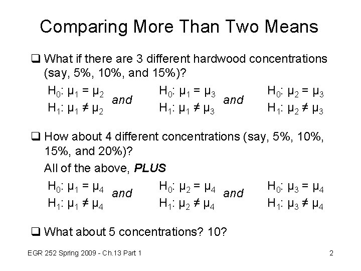
Comparing More Than Two Means q What if there are 3 different hardwood concentrations (say, 5%, 10%, and 15%)? H 0: μ 1 = μ 2 H 0: μ 1 = μ 3 H 0: μ 2 = μ 3 and H 1: μ 1 ≠ μ 2 H 1: μ 2 ≠ μ 3 H 1: μ 1 ≠ μ 3 q How about 4 different concentrations (say, 5%, 10%, 15%, and 20%)? All of the above, PLUS H 0: μ 1 = μ 4 H 0: μ 2 = μ 4 H 0: μ 3 = μ 4 and H 1: μ 1 ≠ μ 4 H 1: μ 2 ≠ μ 4 H 1: μ 3 ≠ μ 4 q What about 5 concentrations? 10? EGR 252 Spring 2009 - Ch. 13 Part 1 2

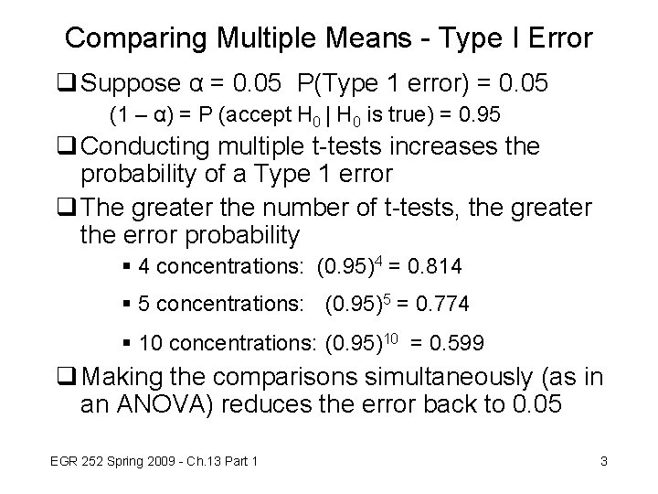
Comparing Multiple Means - Type I Error q Suppose α = 0. 05 P(Type 1 error) = 0. 05 (1 – α) = P (accept H 0 | H 0 is true) = 0. 95 q Conducting multiple t-tests increases the probability of a Type 1 error q The greater the number of t-tests, the greater the error probability § 4 concentrations: (0. 95)4 = 0. 814 § 5 concentrations: (0. 95)5 = 0. 774 § 10 concentrations: (0. 95)10 = 0. 599 q Making the comparisons simultaneously (as in an ANOVA) reduces the error back to 0. 05 EGR 252 Spring 2009 - Ch. 13 Part 1 3

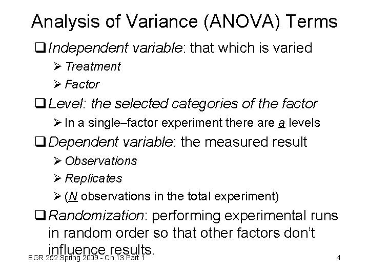
Analysis of Variance (ANOVA) Terms q Independent variable: that which is varied Ø Treatment Ø Factor q Level: the selected categories of the factor Ø In a single–factor experiment there a levels q Dependent variable: the measured result Ø Observations Ø Replicates Ø (N observations in the total experiment) q Randomization: performing experimental runs in random order so that other factors don’t influence results. EGR 252 Spring 2009 - Ch. 13 Part 1 4

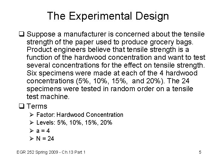
The Experimental Design q Suppose a manufacturer is concerned about the tensile strength of the paper used to produce grocery bags. Product engineers believe that tensile strength is a function of the hardwood concentration and want to test several concentrations for the effect on tensile strength. Six specimens were made at each of the 4 hardwood concentrations (5%, 10%, 15%, and 20%). The 24 specimens were tested in random order on a tensile test machine. q Terms Ø Ø Factor: Hardwood Concentration Levels: 5%, 10%, 15%, 20% a = 4 N = 24 EGR 252 Spring 2009 - Ch. 13 Part 1 5

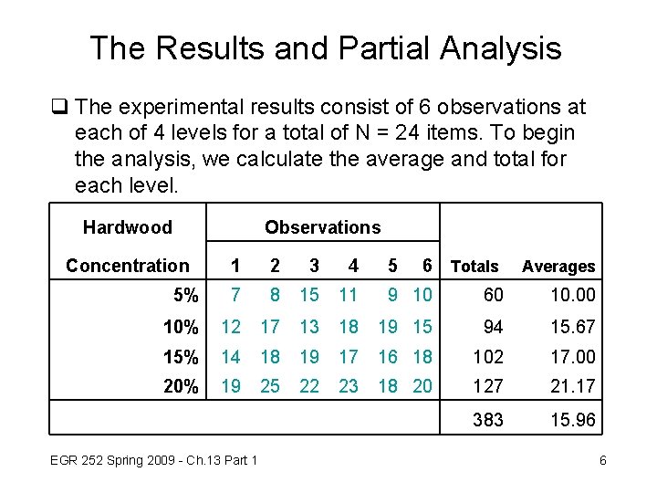
The Results and Partial Analysis q The experimental results consist of 6 observations at each of 4 levels for a total of N = 24 items. To begin the analysis, we calculate the average and total for each level. Hardwood Observations Concentration 1 2 3 4 5 6 Totals 5% 7 8 15 11 9 10 60 10. 00 10% 12 17 13 18 19 15 94 15. 67 15% 14 18 19 17 16 18 102 17. 00 20% 19 25 22 23 18 20 127 21. 17 383 15. 96 EGR 252 Spring 2009 - Ch. 13 Part 1 Averages 6

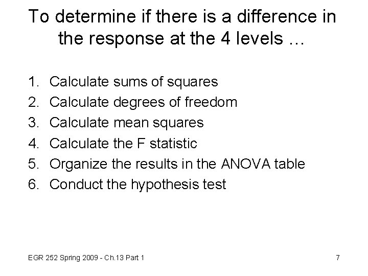
To determine if there is a difference in the response at the 4 levels … 1. 2. 3. 4. 5. 6. Calculate sums of squares Calculate degrees of freedom Calculate mean squares Calculate the F statistic Organize the results in the ANOVA table Conduct the hypothesis test EGR 252 Spring 2009 - Ch. 13 Part 1 7

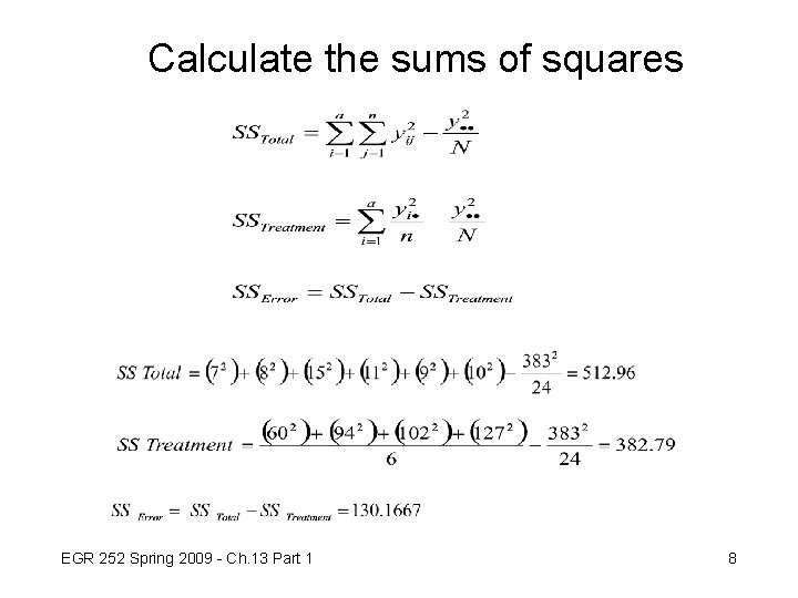
Calculate the sums of squares EGR 252 Spring 2009 - Ch. 13 Part 1 8

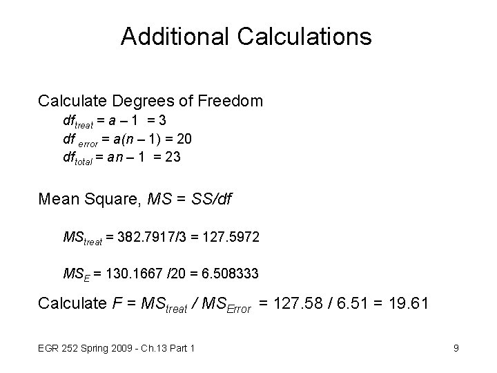
Additional Calculations Calculate Degrees of Freedom dftreat = a – 1 = 3 df error = a(n – 1) = 20 dftotal = an – 1 = 23 Mean Square, MS = SS/df MStreat = 382. 7917/3 = 127. 5972 MSE = 130. 1667 /20 = 6. 508333 Calculate F = MStreat / MSError = 127. 58 / 6. 51 = 19. 61 EGR 252 Spring 2009 - Ch. 13 Part 1 9

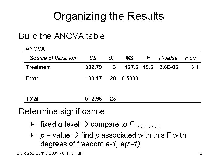
Organizing the Results Build the ANOVA table ANOVA Source of Variation SS df MS Treatment 382. 79 3 Error 130. 17 20 Total 512. 96 23 F 127. 6 19. 6 P-value F crit 3. 6 E-06 3. 1 6. 5083 Determine significance Ø fixed α-level compare to Fα, a-1, a(n-1) Ø p – value find p associated with this F with degrees of freedom a-1, a(n-1) EGR 252 Spring 2009 - Ch. 13 Part 1 10

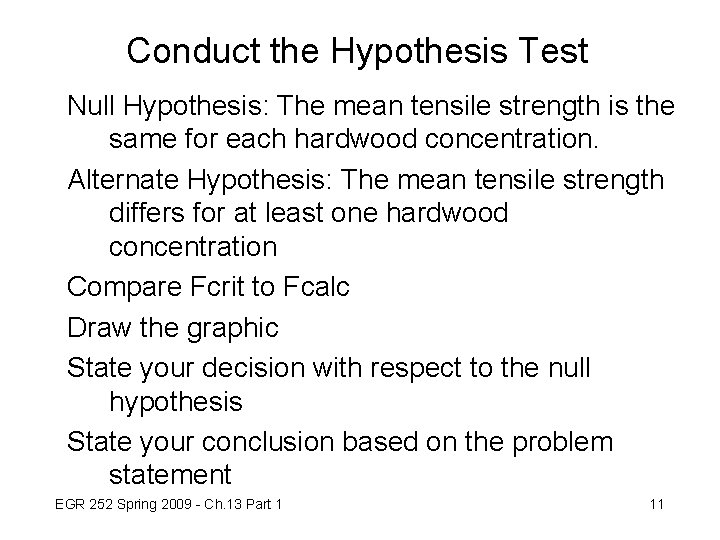
Conduct the Hypothesis Test Null Hypothesis: The mean tensile strength is the same for each hardwood concentration. Alternate Hypothesis: The mean tensile strength differs for at least one hardwood concentration Compare Fcrit to Fcalc Draw the graphic State your decision with respect to the null hypothesis State your conclusion based on the problem statement EGR 252 Spring 2009 - Ch. 13 Part 1 11

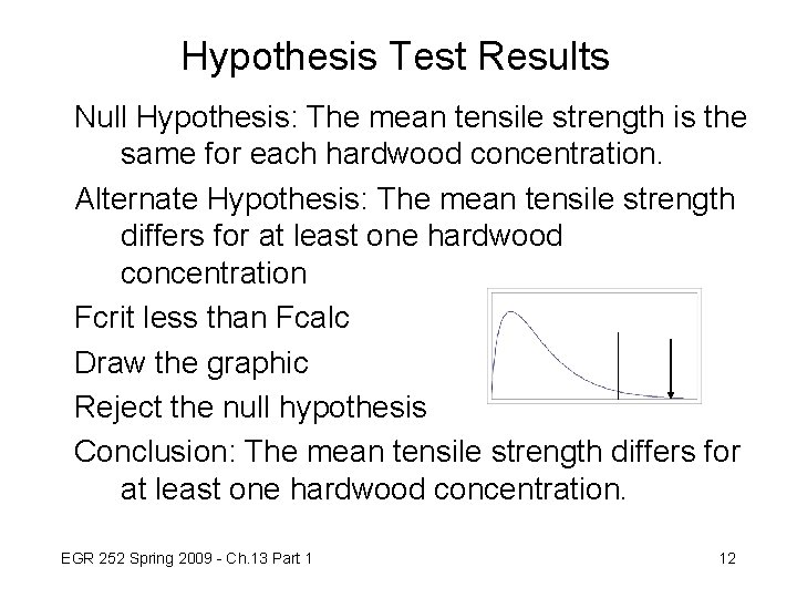
Hypothesis Test Results Null Hypothesis: The mean tensile strength is the same for each hardwood concentration. Alternate Hypothesis: The mean tensile strength differs for at least one hardwood concentration Fcrit less than Fcalc Draw the graphic Reject the null hypothesis Conclusion: The mean tensile strength differs for at least one hardwood concentration. EGR 252 Spring 2009 - Ch. 13 Part 1 12

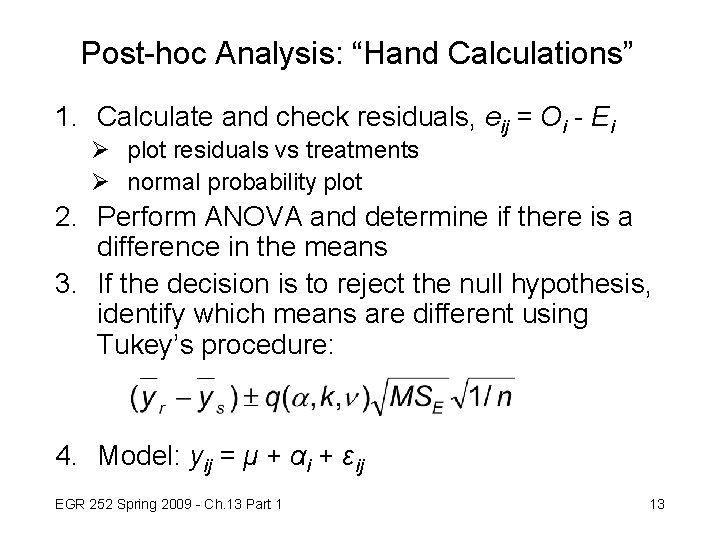
Post-hoc Analysis: “Hand Calculations” 1. Calculate and check residuals, eij = Oi - Ei Ø plot residuals vs treatments Ø normal probability plot 2. Perform ANOVA and determine if there is a difference in the means 3. If the decision is to reject the null hypothesis, identify which means are different using Tukey’s procedure: 4. Model: yij = μ + αi + εij EGR 252 Spring 2009 - Ch. 13 Part 1 13

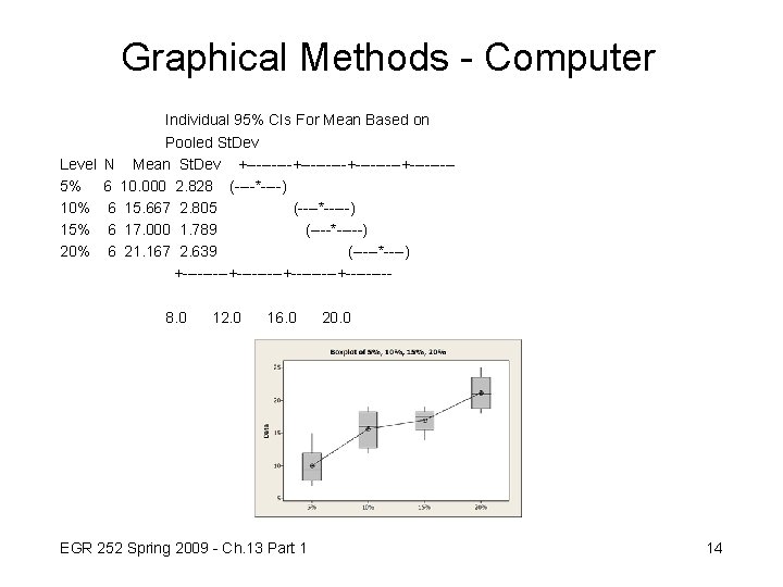
Graphical Methods - Computer Individual 95% CIs For Mean Based on Pooled St. Dev Level N Mean St. Dev +---------+-----+----5% 6 10. 000 2. 828 (----*----) 10% 6 15. 667 2. 805 (----*-----) 15% 6 17. 000 1. 789 (----*-----) 20% 6 21. 167 2. 639 (-----*----) +---------+-----+---- 8. 0 12. 0 16. 0 20. 0 EGR 252 Spring 2009 - Ch. 13 Part 1 14

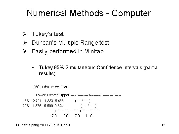
Numerical Methods - Computer Ø Tukey’s test Ø Duncan’s Multiple Range test Ø Easily performed in Minitab § Tukey 95% Simultaneous Confidence Intervals (partial results) 10% subtracted from: Lower Center Upper ----+---------+-----+----15% -2. 791 1. 333 5. 458 (-----*-----) 20% 1. 376 5. 500 9. 624 (-----*-----) ----+---------+-----+---- -7. 0 0. 0 7. 0 14. 0 EGR 252 Spring 2009 - Ch. 13 Part 1 15