Chapter 7 Quantitative Process Analysis Contents SEITE 1

Chapter 7: Quantitative Process Analysis Contents SEITE 1 1. Flow Analysis 2. Queuing Analysis 3. Simulation 4. Recap

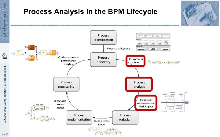
Process Analysis in the BPM Lifecycle

Chapter 7: Quantitative Process Analysis Contents SEITE 3 1. Flow Analysis 2. Queuing Analysis 3. Simulation 4. Recap

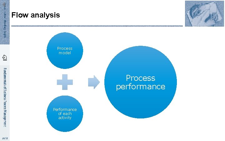
4 Flow analysis Process model Process performance Performance of each activity

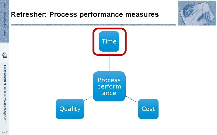
Refresher: Process performance measures Time Process perform ance Quality Cost

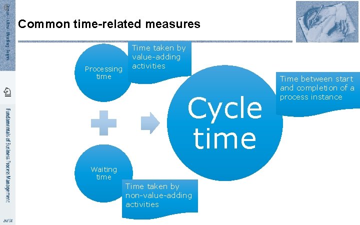
6 Common time-related measures Processing time Time taken by value-adding activities Cycle time Waiting time Time taken by non-value-adding activities Time between start and completion of a process instance

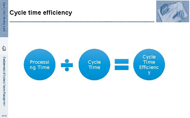
7 Cycle time efficiency Processi ng Time Cycle Time Efficienc y

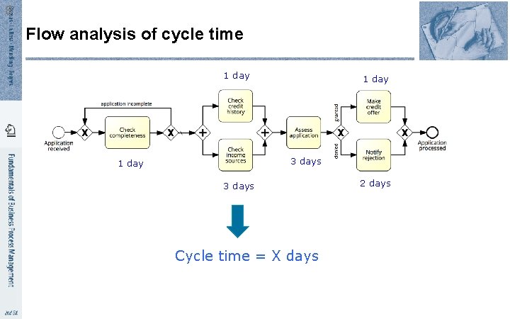
8 Flow analysis of cycle time 1 day 3 days Cycle time = X days 2 days

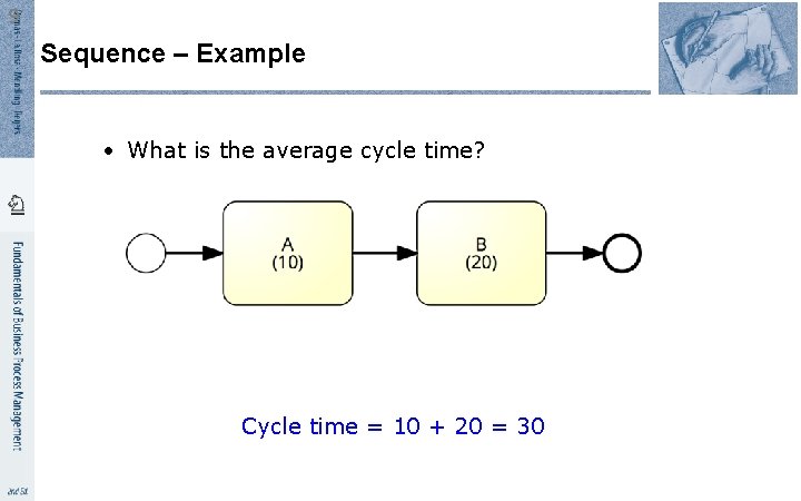
9 Sequence – Example • What is the average cycle time? Cycle time = 10 + 20 = 30

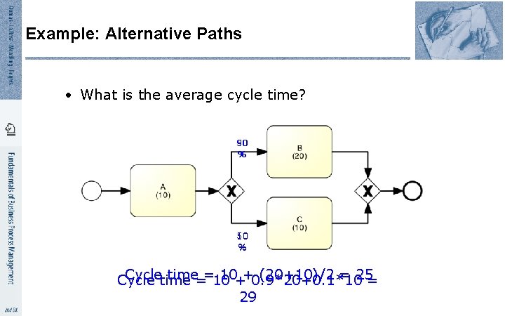
Example: Alternative Paths • What is the average cycle time? 50 90 % 50 10 % Cycletime==10 10++0. 9*20+0. 1*10 (20+10)/2 = 25= Cycle 29

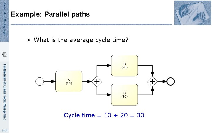
Example: Parallel paths • What is the average cycle time? Cycle time = 10 + 20 = 30

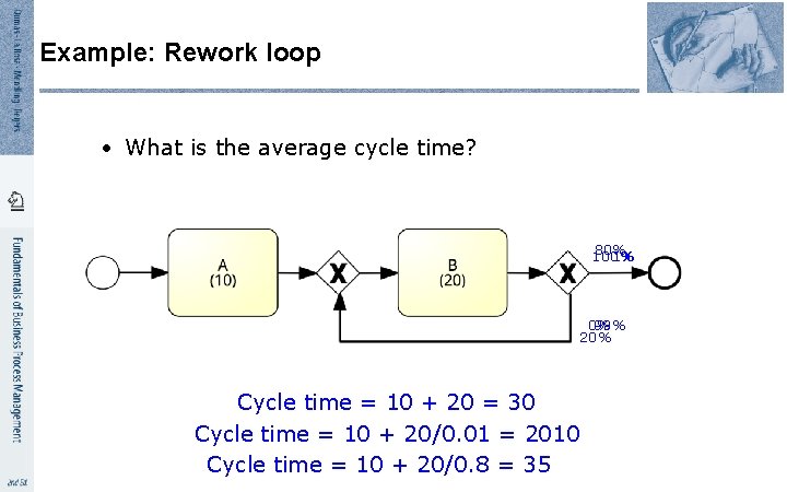
Example: Rework loop • What is the average cycle time? 80% 100% 1% 0% 99% 20% Cycle time = 10 + 20 = 30 Cycle time = 10 + 20/0. 01 = 2010 Cycle time = 10 + 20/0. 8 = 35

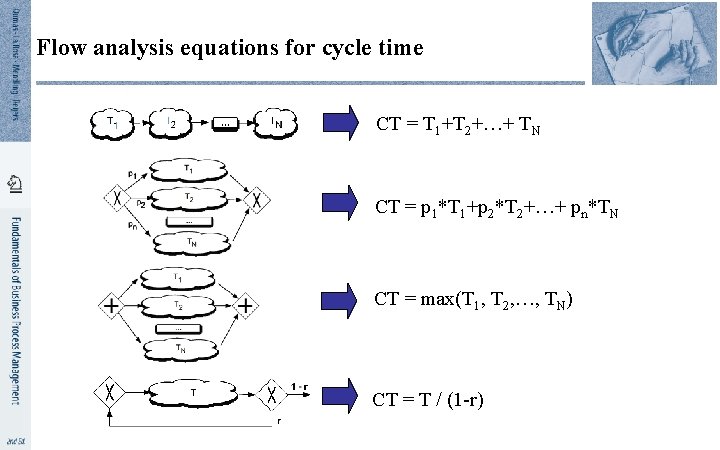
Flow analysis equations for cycle time CT = T 1+T 2+…+ TN CT = p 1*T 1+p 2*T 2+…+ pn*TN CT = max(T 1, T 2, …, TN) CT = T / (1 -r)

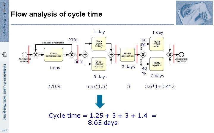
1 4 Flow analysis of cycle time 1 day 20% 60 % 80% 3 days 1 day 3 days 1/0. 8 max(1, 3) 3 40 % 2 days 0. 6*1+0. 4*2 Cycle time = 1. 25 + 3 + 1. 4 = 8. 65 days

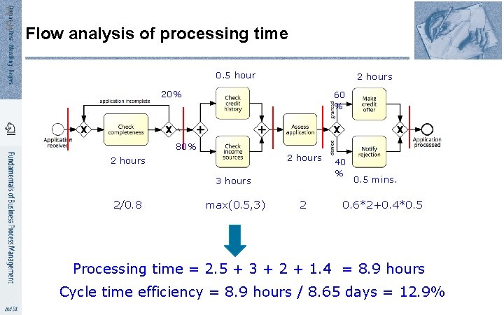
1 5 Flow analysis of processing time 0. 5 hour 2 hours 20% 60 % 80% 2 hours 3 hours 2/0. 8 max(0. 5, 3) 2 40 % 0. 5 mins. 0. 6*2+0. 4*0. 5 Processing time = 2. 5 + 3 + 2 + 1. 4 = 8. 9 hours Cycle time efficiency = 8. 9 hours / 8. 65 days = 12. 9%

Flow analysis: scope and limitations § We have seen how to use flow analysis for processing & cycle time calculation § Flow analysis can also be applied to calculate: § The average cost of process instances (assuming we know the cost of each activity) § Cf. Section 7. 1. 6 § The number of times on average each activity is executed § § Can be used to calculate the “unit load” of each task, the resource utilization of each resource pool, and theoretical capacity of an “as is” process Cf. Section 7. 1. 5 § But flow analysis has some fundamental limitations…

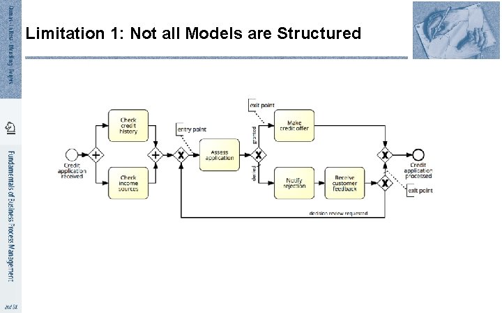
Limitation 1: Not all Models are Structured

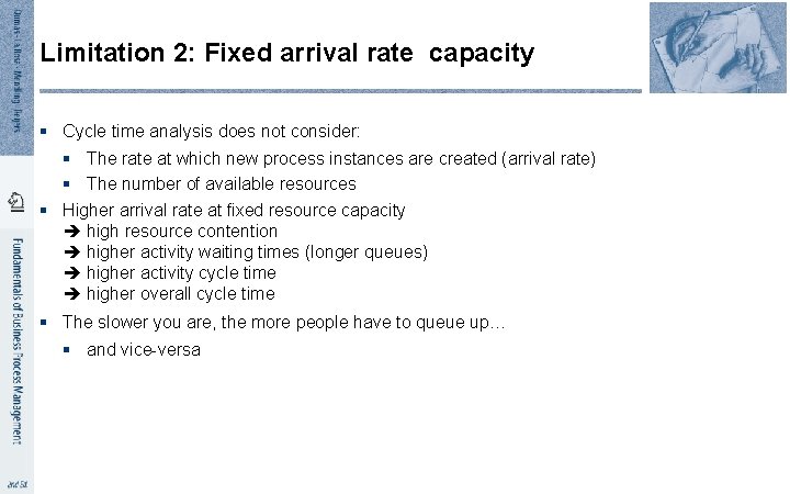
Limitation 2: Fixed arrival rate capacity § Cycle time analysis does not consider: § The rate at which new process instances are created (arrival rate) § The number of available resources § Higher arrival rate at fixed resource capacity high resource contention higher activity waiting times (longer queues) higher activity cycle time higher overall cycle time § The slower you are, the more people have to queue up… § and vice-versa

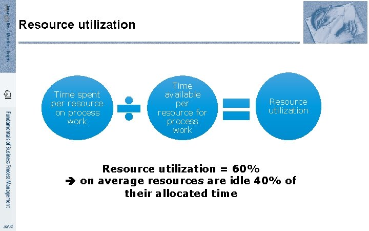
1 9 Resource utilization Time spent per resource on process work Time available per resource for process work Resource utilization = 60% on average resources are idle 40% of their allocated time

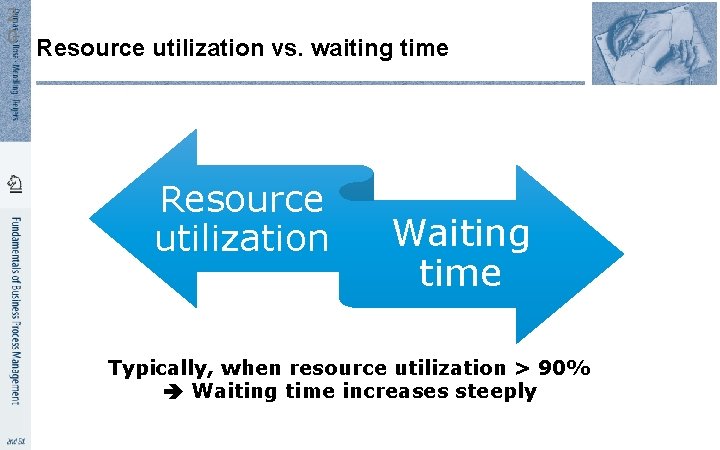
2 0 Resource utilization vs. waiting time Resource utilization Waiting time Typically, when resource utilization > 90% Waiting time increases steeply

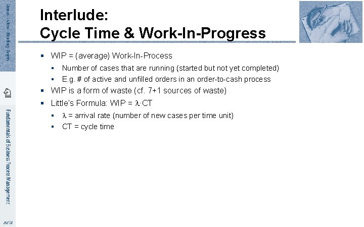
Interlude: Cycle Time & Work-In-Progress § WIP = (average) Work-In-Process § Number of cases that are running (started but not yet completed) § E. g. # of active and unfilled orders in an order-to-cash process § WIP is a form of waste (cf. 7+1 sources of waste) § Little’s Formula: WIP = ·CT § = arrival rate (number of new cases per time unit) § CT = cycle time

Exercise A fast-food restaurant receives on average 1200 customers per day (between 10: 00 and 22: 00). During peak times (12: 00 -15: 00 and 18: 00 -21: 00), the restaurant receives around 900 customers in total, and 90 customers can be found in the restaurant (on average) at a given point in time. At non-peak times, the restaurant receives 300 customers in total, and 30 customers can be found in the restaurant (on average) at a given point in time. 1. What is the average time that a customer spends in the restaurant during peak times? 2. What is the average time that a customer spends in the restaurant during non-peak times?

Exercise (cont. ) 3. The restaurant plans to launch a marketing campaign to attract more customers. However, the restaurant’s capacity is limited and becomes too full during peak times. What can the restaurant do to address this issue without investing in extending its building?

Chapter 7: Quantitative Process Analysis Contents SEITE 24 1. Flow Analysis 2. Queuing Analysis 3. Simulation 4. Recap

2 5 Queuing Analysis § Capacity problems are common and a key driver of process redesign § Need to balance the cost of increased capacity against the gains of increased productivity and service § Queuing and waiting time analysis is particularly important in service systems § Large costs of waiting and/or lost sales due to waiting § Example – Emergency Room (ER) at a Hospital § § Patients arrive by ambulance or by their own accord One doctor is always on duty More patients seeks help longer waiting times Should we increase the capacity from one to two doctors? Inspired by an example by Laguna & Marklund (2004)

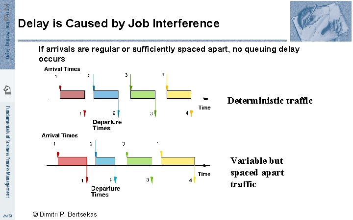
2 6 Delay is Caused by Job Interference If arrivals are regular or sufficiently spaced apart, no queuing delay occurs Deterministic traffic Variable but spaced apart traffic © Dimitri P. Bertsekas

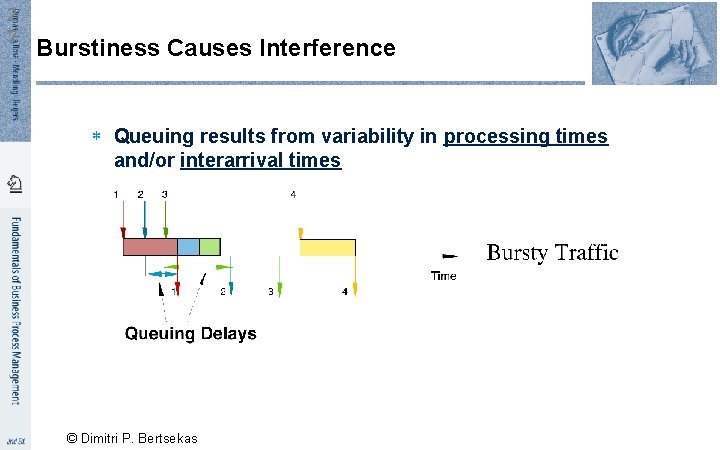
2 7 Burstiness Causes Interference Queuing results from variability in processing times and/or interarrival times © Dimitri P. Bertsekas

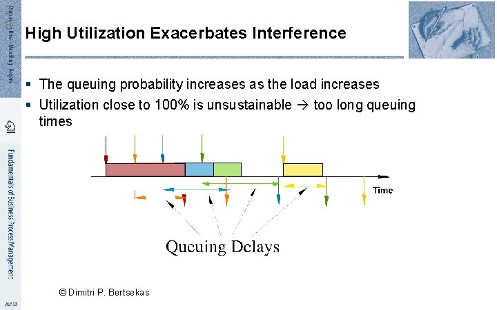
2 8 High Utilization Exacerbates Interference § The queuing probability increases as the load increases § Utilization close to 100% is unsustainable too long queuing times © Dimitri P. Bertsekas

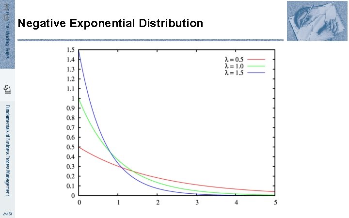
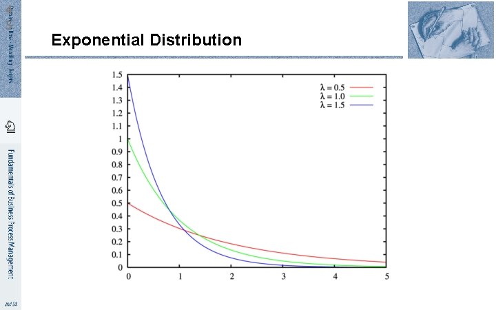
2 9 The Poisson Process § Common arrival assumption in many queuing and simulation models § The times between arrivals are independent, identically distributed and exponential § P (arrival < t) = 1 – e-λt § This distribution is applicable when the next arrival (i. e. the next creation of a case) does not depend on how long ago the previous arrival occurred § In other words, the creation of a case is independent of the creation of other cases. Inspired by slide by Laguna & Marklund (2004)

3 0 Negative Exponential Distribution

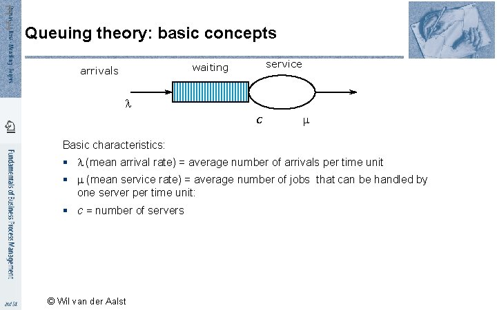
3 1 Queuing theory: basic concepts service waiting arrivals c Basic characteristics: § (mean arrival rate) = average number of arrivals per time unit § (mean service rate) = average number of jobs that can be handled by one server per time unit: § c = number of servers © Wil van der Aalst

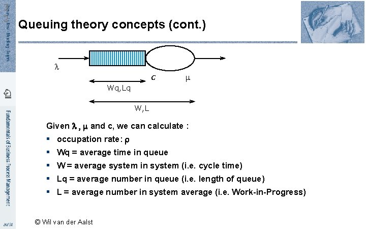
3 2 Queuing theory concepts (cont. ) c Wq, Lq W, L Given , and c, we can calculate : § occupation rate: § Wq = average time in queue § W = average system in system (i. e. cycle time) § Lq = average number in queue (i. e. length of queue) § L = average number in system average (i. e. Work-in-Progress) © Wil van der Aalst

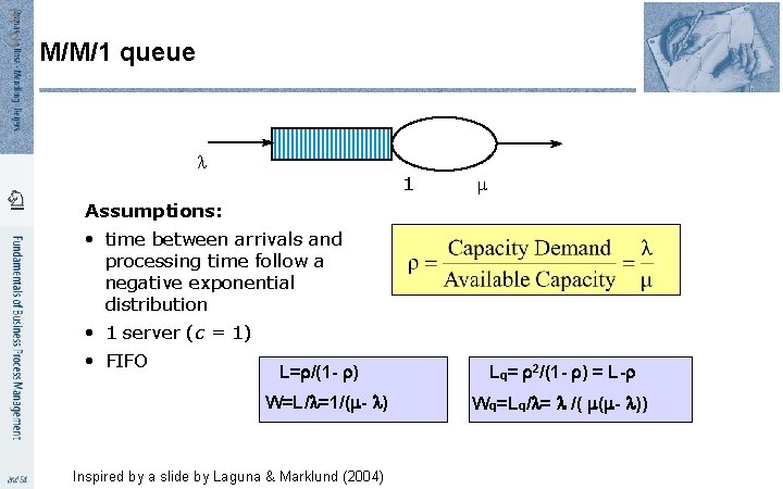
3 3 M/M/1 queue 1 Assumptions: • time between arrivals and processing time follow a negative exponential distribution • 1 server (c = 1) • FIFO L= /(1 - ) W=L/ =1/( - ) Inspired by a slide by Laguna & Marklund (2004) Lq= 2/(1 - ) = L- Wq=Lq/ = /( ( - ))

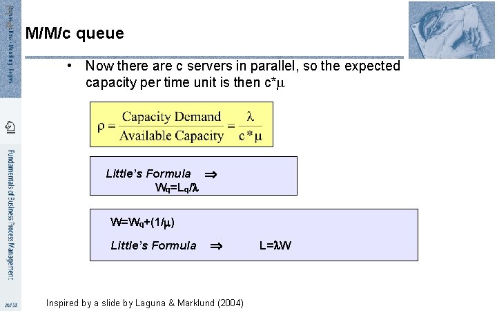
3 4 M/M/c queue • Now there are c servers in parallel, so the expected capacity per time unit is then c* Little’s Formula Wq=Lq/ W=Wq+(1/ ) Little’s Formula Inspired by a slide by Laguna & Marklund (2004) L= W

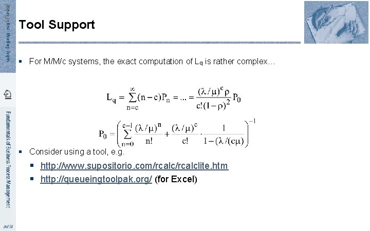
3 5 Tool Support § For M/M/c systems, the exact computation of Lq is rather complex… § Consider using a tool, e. g. § http: //www. supositorio. com/rcalclite. htm § http: //queueingtoolpak. org/ (for Excel)

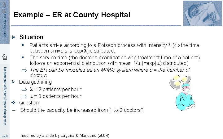
3 6 Example – ER at County Hospital Ø Situation Patients arrive according to a Poisson process with intensity ( the time between arrivals is exp( ) distributed. § The service time (the doctor’s examination and treatment time of a patient) follows an exponential distribution with mean 1/ (=exp( ) distributed) The ER can be modeled as an M/M/c system where c = the number of doctors Ø Data gathering = 2 patients per hour = 3 patients per hour v Question – Should the capacity be increased from 1 to 2 doctors? § Inspired by a slide by Laguna & Marklund (2004)

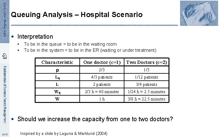
3 7 Queuing Analysis – Hospital Scenario § Interpretation § To be in the queue = to be in the waiting room § To be in the system = to be in the ER (waiting or under treatment) Characteristic One doctor (c=1) Two Doctors (c=2) 2/3 1/3 Lq 4/3 patients 1/12 patients L 2 patients 3/4 patients Wq 2/3 h = 40 minutes 1/24 h = 2. 5 minutes W 1 h 3/8 h = 22. 5 minutes § Should we increase the capacity from one to two doctors? Inspired by a slide by Laguna & Marklund (2004)

3 8 Limitations of basic queuing models § Can be used to analyze waiting times (and hence cycle times), but not cost or quality measures § Suitable for analyzing one single activity at a time, performed by one single resource pool. Not suitable for analyzing end-to-end processes consisting of multiple activities performed by multiple resource pools. § These limitations are addressed by process simulation

Chapter 7: Quantitative Process Analysis Contents SEITE 39 1. Value-Added Analysis 2. Queuing analysis 3. Simulation 4. Recap

4 0 Process Simulation § Versatile quantitative analysis method for § As-is analysis § What-if analysis § In a nutshell: § Run a large number of process instances § Gather performance data (cost, time, resource usage) § Calculate statistics from the collected data

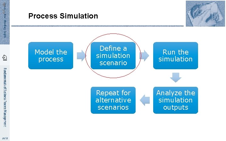
4 1 Process Simulation Model the process Define a simulation scenario Run the simulation Repeat for alternative scenarios Analyze the simulation outputs

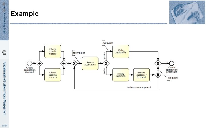
4 2 Example

4 3 Example

4 4 Elements of a simulation scenario 1. Processing times of activities § Fixed value § Probability distribution

4 5 Exponential Distribution

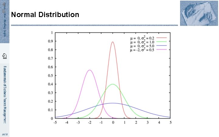
4 6 Normal Distribution

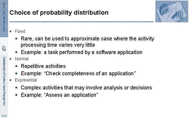
4 7 Choice of probability distribution § Fixed § Rare, can be used to approximate case where the activity processing time varies very little § Example: a task performed by a software application § Normal § Repetitive activities § Example: “Check completeness of an application” § Exponential § Complex activities that may involve analysis or decisions § Example: “Assess an application”

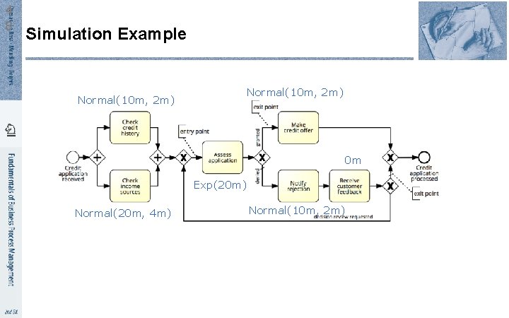
4 8 Simulation Example Normal(10 m, 2 m) 0 m Exp(20 m) Normal(20 m, 4 m) Normal(10 m, 2 m)

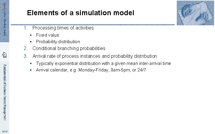
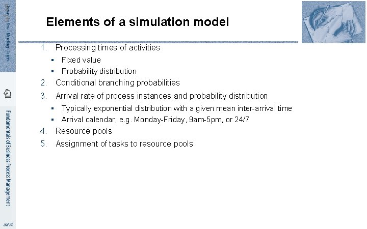
4 9 Elements of a simulation model 1. Processing times of activities § Fixed value § Probability distribution 2. Conditional branching probabilities 3. Arrival rate of process instances and probability distribution § Typically exponential distribution with a given mean inter-arrival time § Arrival calendar, e. g. Monday-Friday, 9 am-5 pm, or 24/7

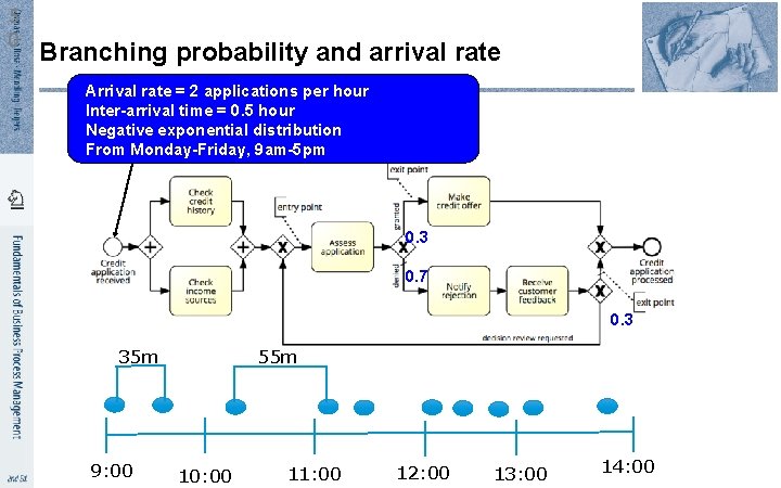
5 0 Branching probability and arrival rate Arrival rate = 2 applications per hour Inter-arrival time = 0. 5 hour Negative exponential distribution From Monday-Friday, 9 am-5 pm 0. 3 0. 7 0. 3 55 m 35 m 9: 00 10: 00 11: 00 12: 00 13: 00 14: 00

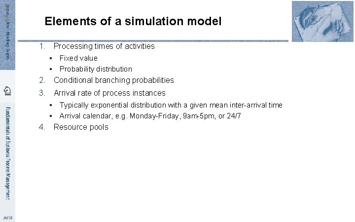
5 1 Elements of a simulation model 1. Processing times of activities § Fixed value § Probability distribution 2. Conditional branching probabilities 3. Arrival rate of process instances § Typically exponential distribution with a given mean inter-arrival time § Arrival calendar, e. g. Monday-Friday, 9 am-5 pm, or 24/7 4. Resource pools

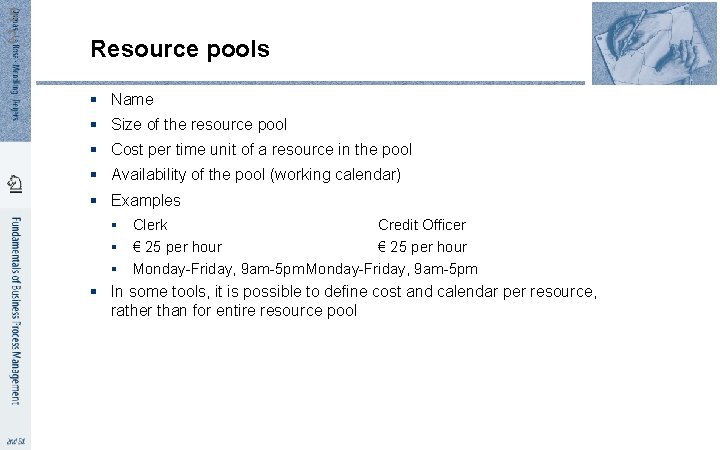
5 2 Resource pools § Name § Size of the resource pool § Cost per time unit of a resource in the pool § Availability of the pool (working calendar) § Examples § Clerk Credit Officer § € 25 per hour § Monday-Friday, 9 am-5 pm § In some tools, it is possible to define cost and calendar per resource, rather than for entire resource pool

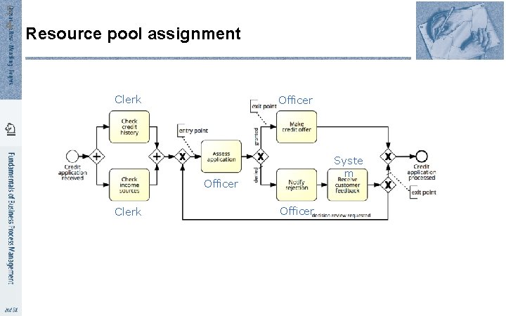
5 3 Elements of a simulation model 1. Processing times of activities § Fixed value § Probability distribution 2. Conditional branching probabilities 3. Arrival rate of process instances and probability distribution § Typically exponential distribution with a given mean inter-arrival time § Arrival calendar, e. g. Monday-Friday, 9 am-5 pm, or 24/7 4. Resource pools 5. Assignment of tasks to resource pools

5 4 Resource pool assignment Clerk Officer Syste m Officer Clerk Officer

5 5 Process Simulation ✔ Model the process ✔ ✔ Define a simulation scenario Run the simulation Repeat for alternative scenarios Analyze the simulation outputs

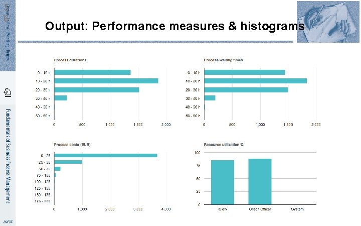
5 6 Output: Performance measures & histograms

5 7 Process Simulation ✔ Model the process ✔ Define a simulation scenario ✔ Run the simulation ✔ Repeat for alternative scenarios Analyze the simulation outputs

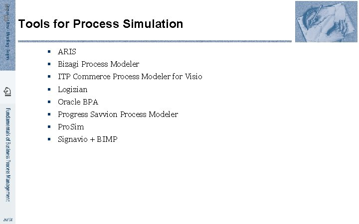
5 8 Tools for Process Simulation § ARIS § Bizagi Process Modeler § ITP Commerce Process Modeler for Visio § Logizian § Oracle BPA § Progress Savvion Process Modeler § Pro. Sim § Signavio + BIMP

5 9 BIMP – bimp. cs. ut. ee § Accepts standard BPMN 2. 0 as input § Simple form-based interface to enter simulation scenario § Produces KPIs + simulation logs in MXML format § Simulation logs can be imported to the Pro. M process mining tool

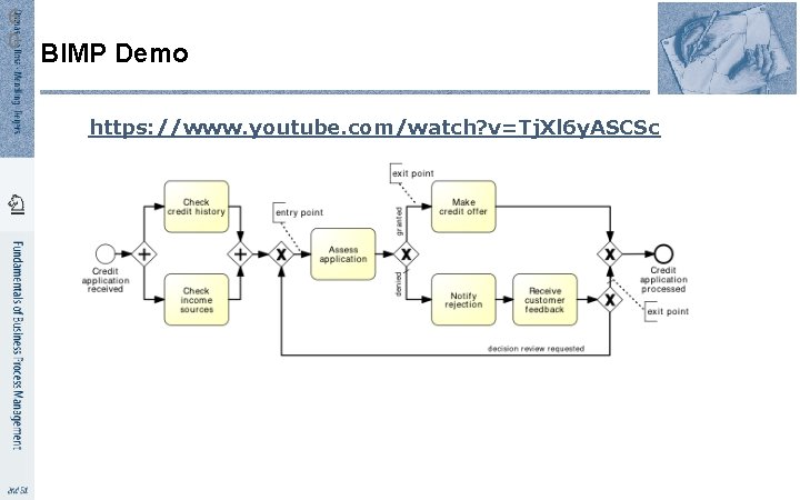
6 0 BIMP Demo https: //www. youtube. com/watch? v=Tj. Xl 6 y. ASCSc

6 1 Pitfalls of simulation § Stochasticity § Data quality pitfalls § Simplifying assumptions

6 2 Stochasticity § Simulation results may differ from one run to another § Make the simulation tiemframe long enough to cover weekly and seasonal variability, where applicable § Use multiple simulation runs § Average results of multiple runs, compute confidence intervals

6 3 Data quality pitfalls § Simulation results are only as trustworthy as the input data § Rely as little as possible on “guesstimates” § Use input analysis § Deriver simulation scenario parameters from numbers in the scenario § Use statistical tools to check fit the probability distributions § Simulate the “as is” scenario and cross-check results against actual observations

6 4 Simulation assumptions § That the process model is always followed to the letter § No deviations § No workarounds § That there is no multi-tasking (the same resource performs multiple tasks concurrently) nor batching (tasks being accumulated and performed in a single go) § That resources work constantly and non-stop § Every day is the same! § No tiredness effects § No distractions beyond “stochastic” ones

Chapter 7: Quantitative Process Analysis Contents SEITE 65 1. Value-Added Analysis 2. Queuing analysis 3. Simulation 4. Recap

Recap § Assuming we have performance measures for each activity in a process, flow analysis allows us to calculate the following performance measures for an “as is” process: § Cycle time, processing times, cycle time efficiency of a process § Average cost per process instance § It can also be used to calculate theoretical capacity of an “as is” process and the resource utilization of resource pools § But it is not suitable for “what if” analysis § Queing analysis is a suitable technique for “what if” analysis of waiting times and cycle times, suitable for analyzing individual activities performed by one resource pool § Simulation is a versatile technique for “what if” analysis of entire processes, covering waiting times, cycle times, and costs. § Particularly useful for identifying bottlenecks SLIDE