A Tour of Image Denoising Shahar Kovalsky Alon

A Tour of Image Denoising Shahar Kovalsky Alon Faktor 17/4/2011

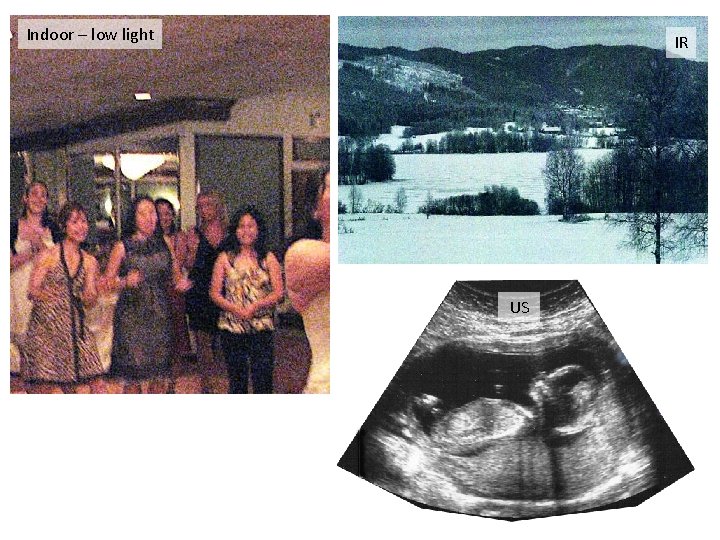
Indoor – low light IR US

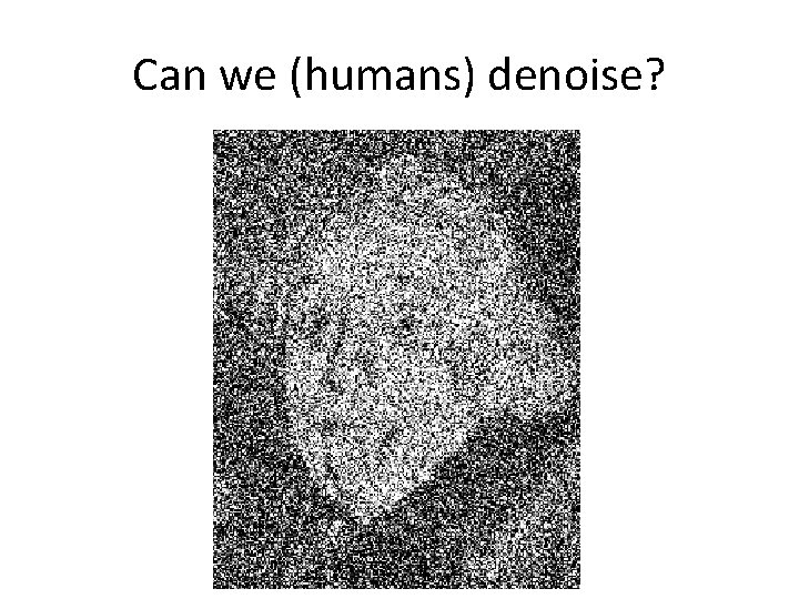
Can we (humans) denoise?

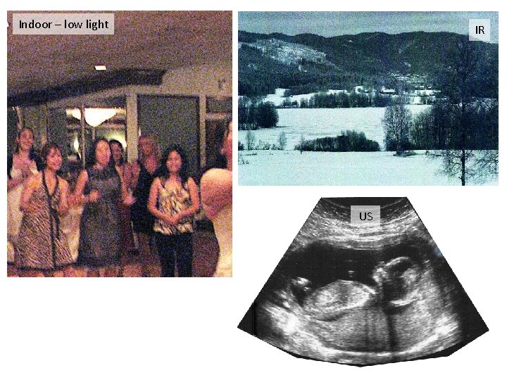
Indoor – low light IR US

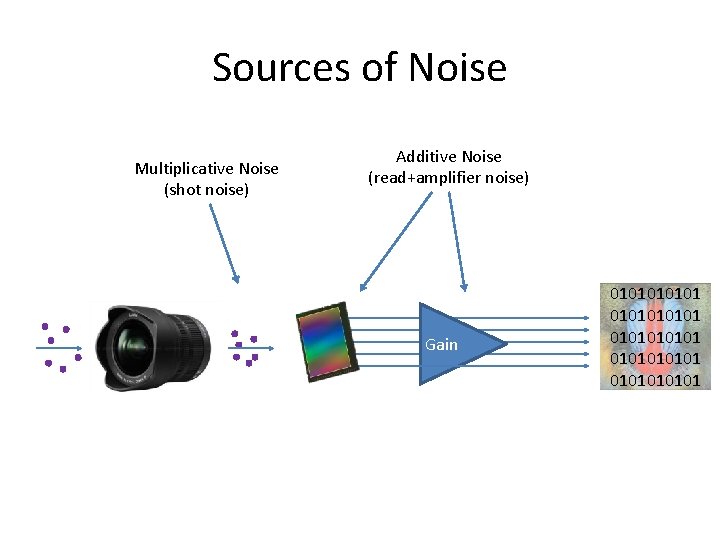
Sources of Noise Multiplicative Noise (shot noise) Additive Noise (read+amplifier noise) Gain 0101010101 010101

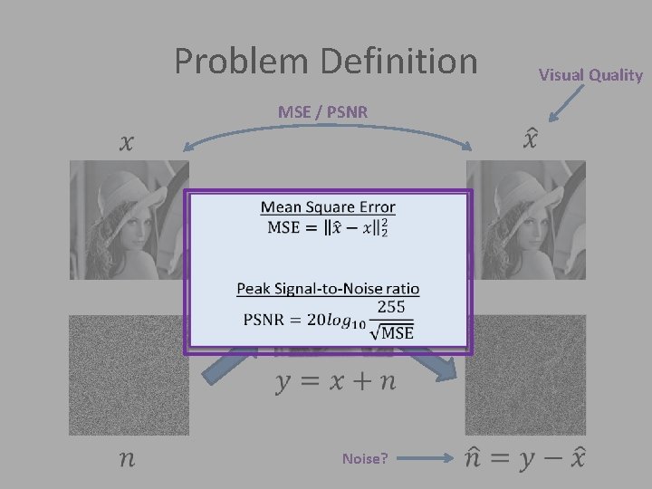
Problem Definition MSE / PSNR Noise? Visual Quality

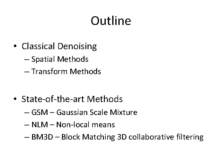
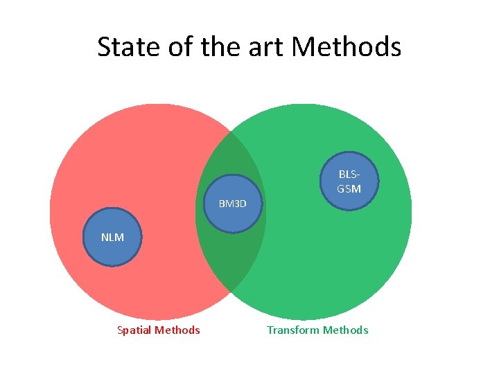
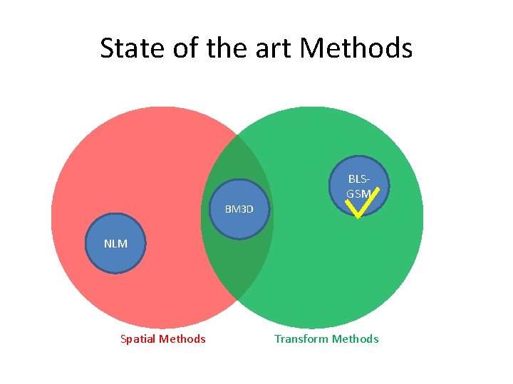
Outline • Classical Denoising – Spatial Methods – Transform Methods • State-of-the-art Methods – GSM – Gaussian Scale Mixture – NLM – Non-local means – BM 3 D – Block Matching 3 D collaborative filtering

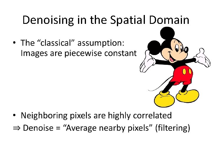
Denoising in the Spatial Domain •

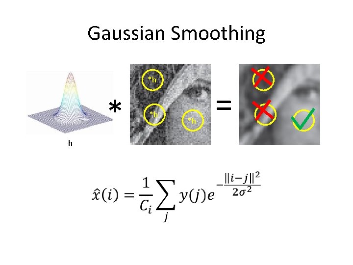
Gaussian Smoothing *h * h • *h *h =

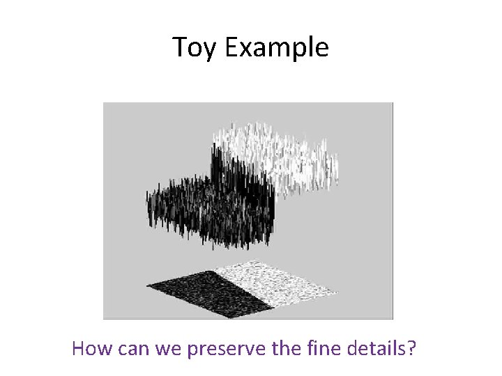
Toy Example How can we preserve the fine details?

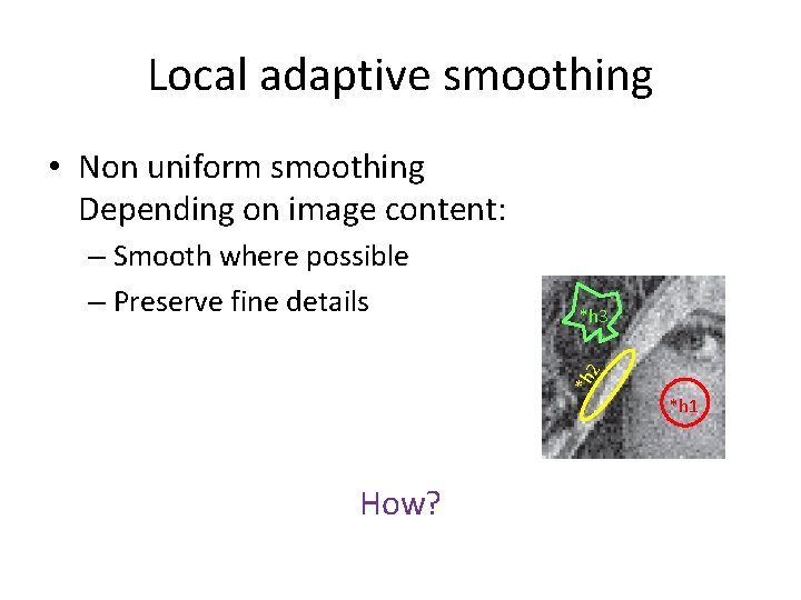
Local adaptive smoothing • Non uniform smoothing Depending on image content: *h 3 *h 2 – Smooth where possible – Preserve fine details *h 1 How?

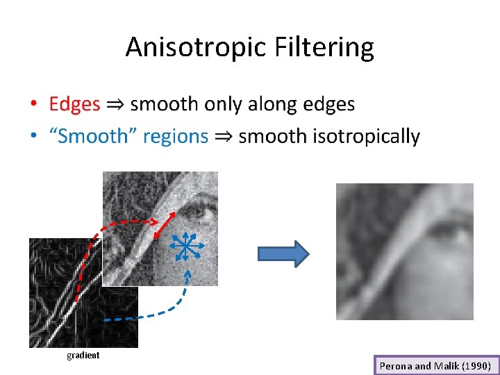
Anisotropic Filtering • gradient Perona and Malik (1990)

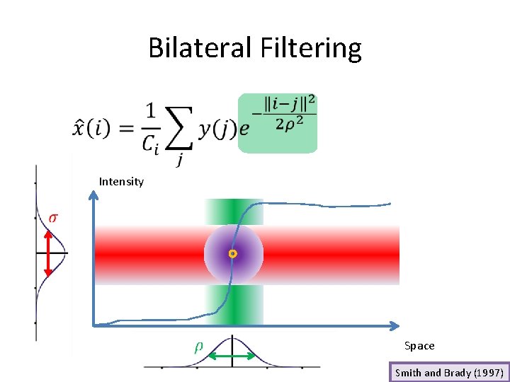
Bilateral Filtering • Intensity Space Smith and Brady (1997)

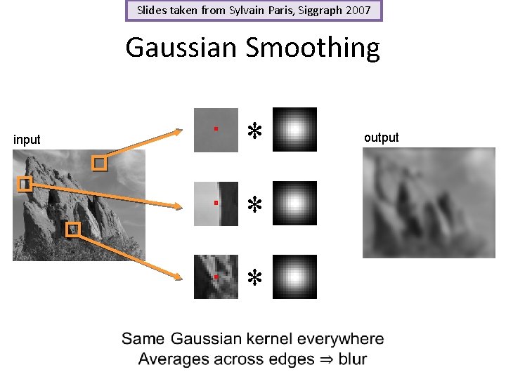
Slides taken from Sylvain Paris, Siggraph 2007 Gaussian Smoothing * input * * output

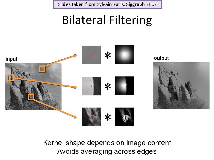
Slides taken from Sylvain Paris, Siggraph 2007 Bilateral Filtering input * output * * Kernel shape depends on image content Avoids averaging across edges

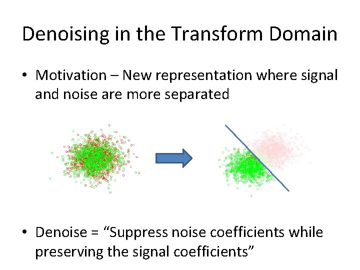
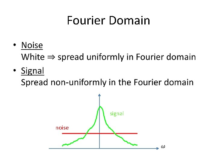
Denoising in the Transform Domain • Motivation – New representation where signal and noise are more separated • Denoise = “Suppress noise coefficients while preserving the signal coefficients”

Fourier Domain • signal noise

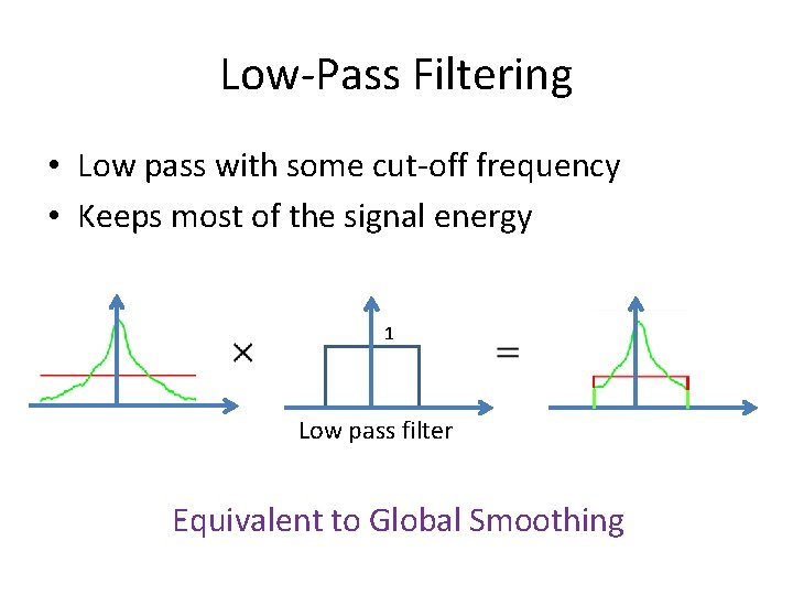
Low-Pass Filtering • Low pass with some cut-off frequency • Keeps most of the signal energy 1 Low pass filter Equivalent to Global Smoothing

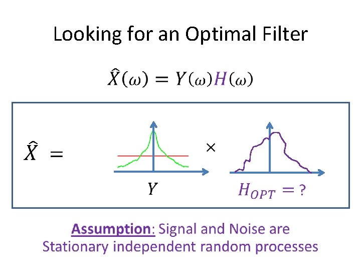
Looking for an Optimal Filter •

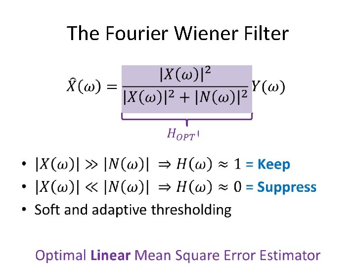
The Fourier Wiener Filter •

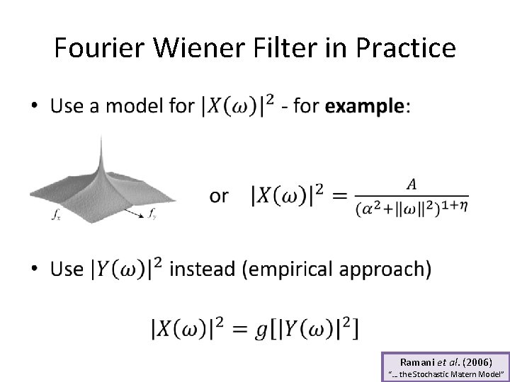
Fourier Wiener Filter in Practice • Ramani et al. (2006) “… the Stochastic Matern Model”

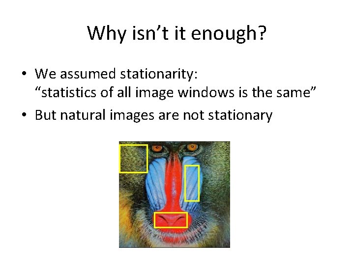
Why isn’t it enough? • We assumed stationarity: “statistics of all image windows is the same” • But natural images are not stationary

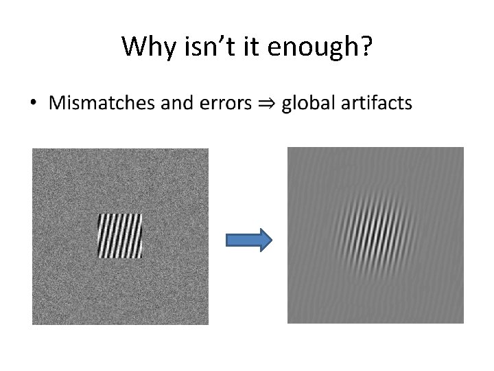
Why isn’t it enough? •

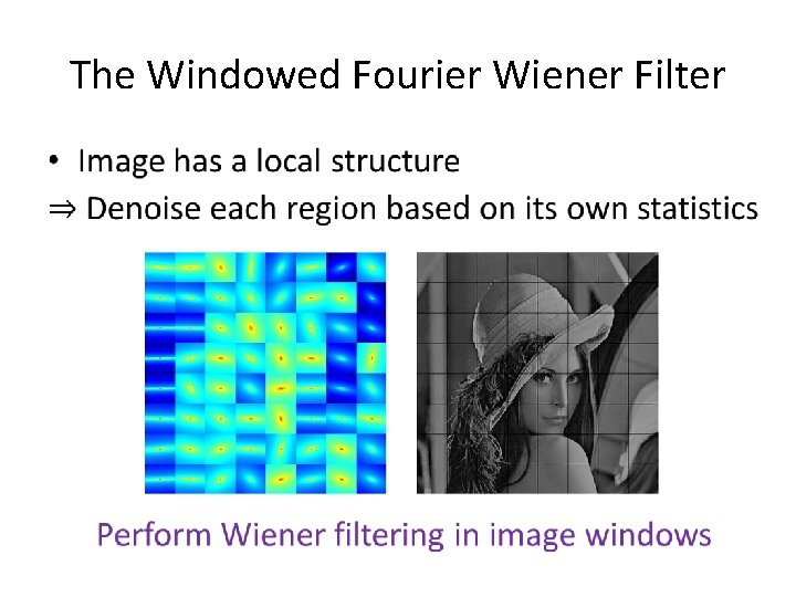
The Windowed Fourier Wiener Filter •

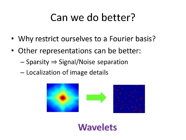
Can we do better? •

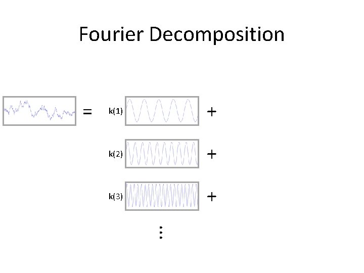
Fourier Decomposition = k(1) + k(2) + k(3) + ···

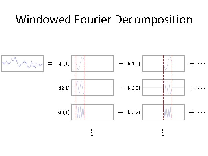
Windowed Fourier Decomposition = k(1, 1) + k(1, 2) + ··· k(2, 1) + k(2, 2) + ··· k(3, 1) + k(3, 2) + ··· ···

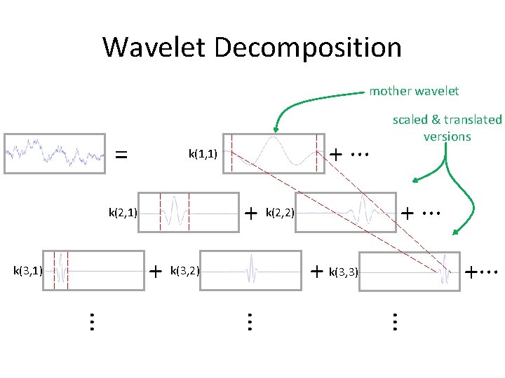
Wavelet Decomposition mother wavelet = + ··· k(1, 1) + k(2, 2) k(2, 1) + k(3, 2) k(3, 1) scaled & translated versions + ··· + k(3, 3) +··· ···

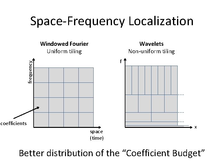
Space-Frequency Localization Windowed Fourier Uniform tiling Wavelets Non-uniform tiling frequency f coefficients space (time) x Better distribution of the “Coefficient Budget”

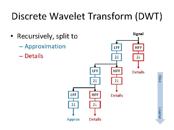
Discrete Wavelet Transform (DWT) Signal • Recursively, split to – Approximation – Details HPF Details Fine Coarse LPF Approx LPF

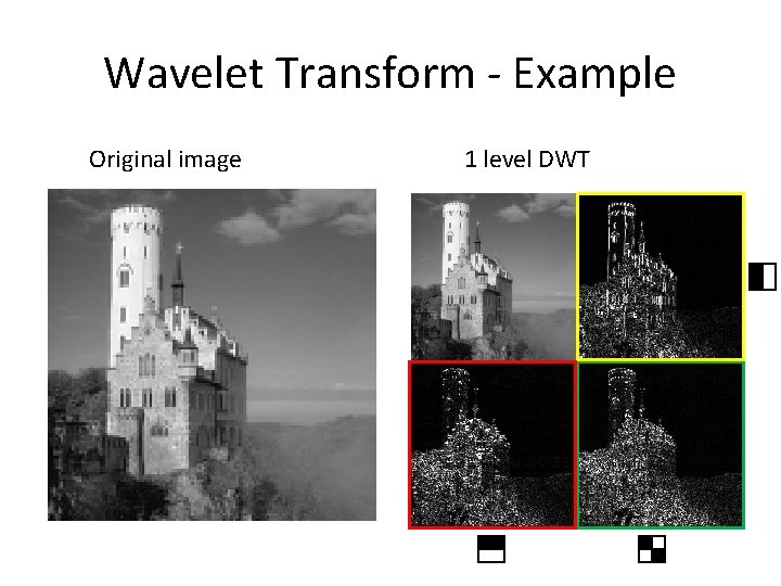
Wavelet Transform - Example Original image 1 level DWT

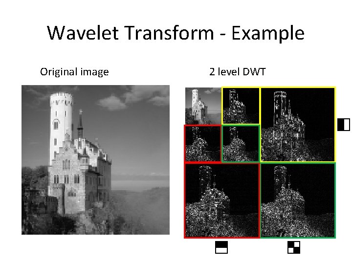
Wavelet Transform - Example Original image 2 level DWT

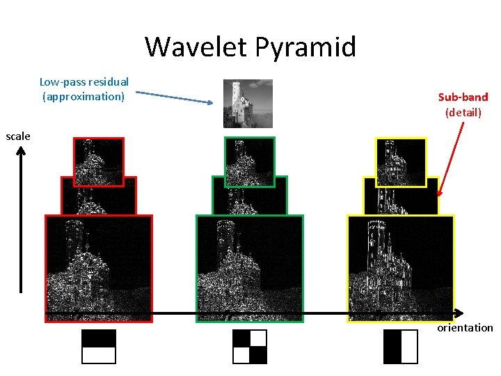
Wavelet Pyramid Low-pass residual (approximation) Sub-band (detail) scale orientation

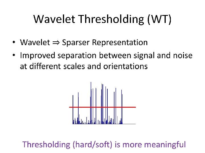
Wavelet Thresholding (WT) •

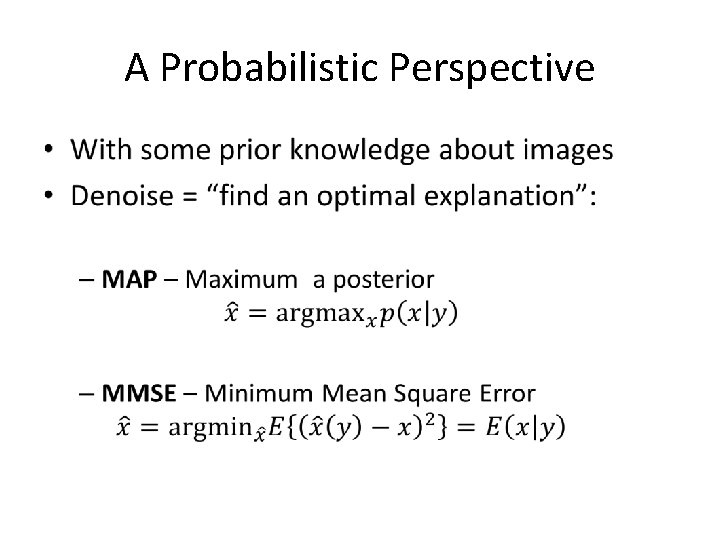
A Probabilistic Perspective •

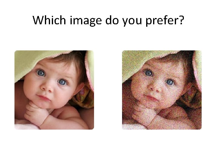
Which image do you prefer?

A Probabilistic Perspective •

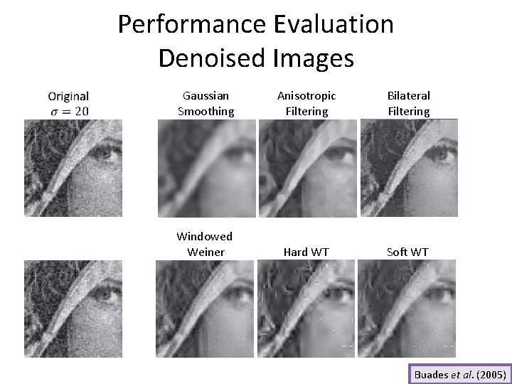
Performance Evaluation Denoised Images Gaussian Smoothing Anisotropic Filtering Bilateral Filtering Windowed Weiner Hard WT Soft WT Buades et al. (2005)

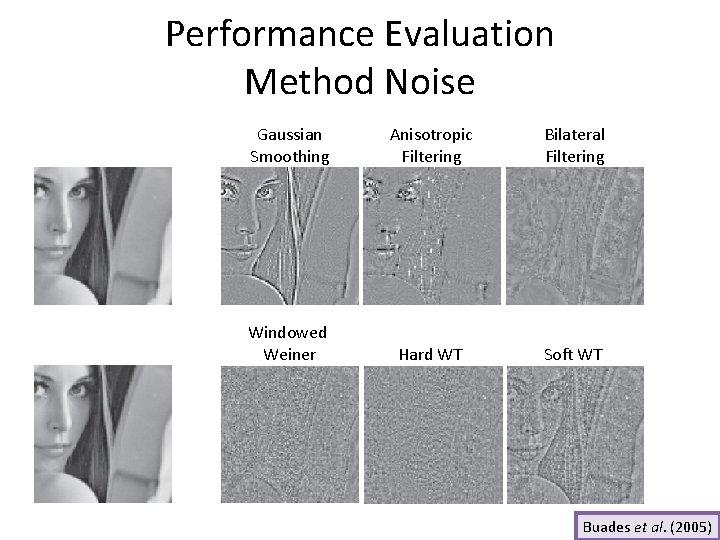
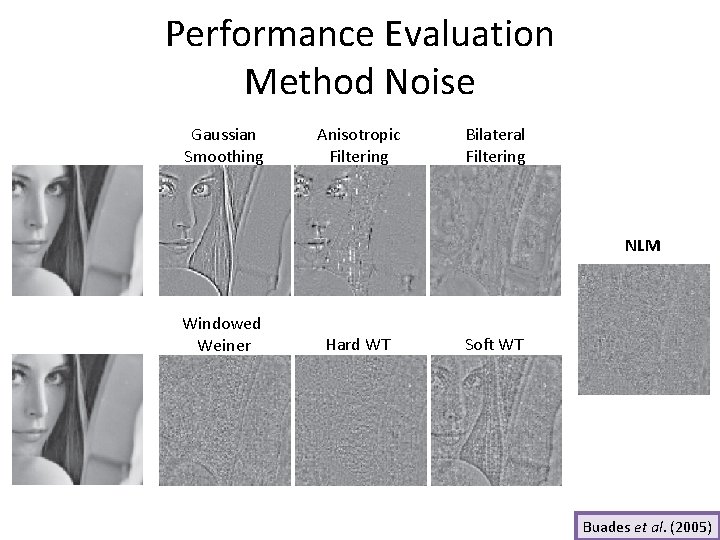
Performance Evaluation Method Noise Gaussian Smoothing Anisotropic Filtering Bilateral Filtering Windowed Weiner Hard WT Soft WT Buades et al. (2005)

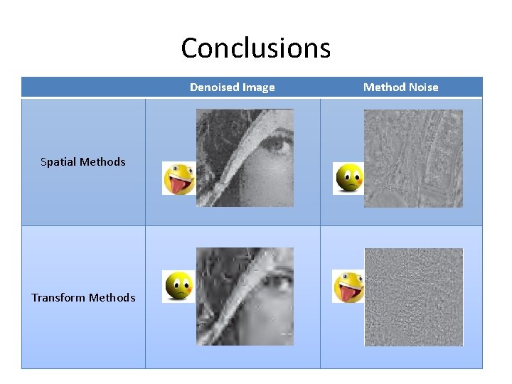
Conclusions Denoised Image Spatial Methods Transform Methods Method Noise

Taking it up a notch. . .

State of the art Methods BLSGSM BM 3 D NLM Spatial Methods Transform Methods

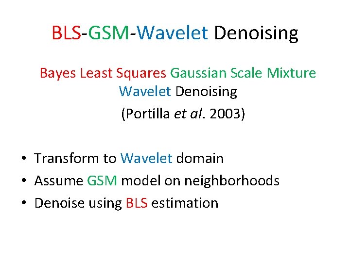
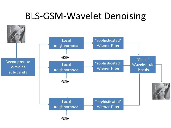
BLS-GSM-Wavelet Denoising Bayes Least Squares Gaussian Scale Mixture Wavelet Denoising (Portilla et al. 2003) • Transform to Wavelet domain • Assume GSM model on neighborhoods • Denoise using BLS estimation

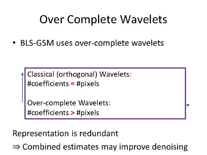
Over Complete Wavelets • Classical (orthogonal) Wavelets: #coefficients = #pixels Over-complete Wavelets: #coefficients > #pixels …

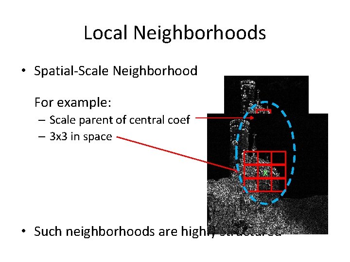
Local Neighborhoods • Spatial-Scale Neighborhood For example: – Scale parent of central coef – 3 x 3 in space x • Such neighborhoods are highly structured

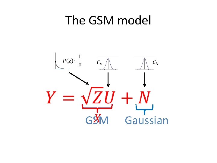
The GSM model GSM Gaussian

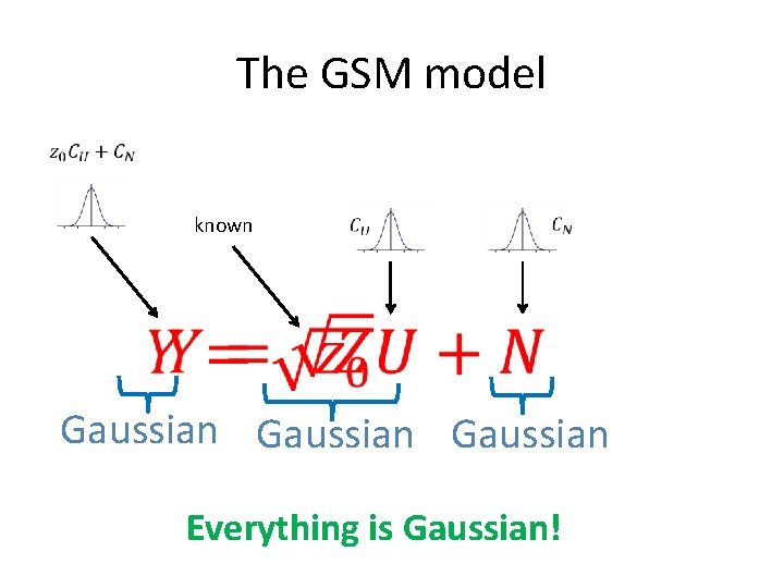
The GSM model known Gaussian Everything is Gaussian!

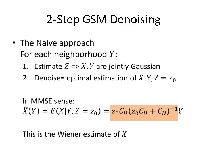
2 -Step GSM Denoising •

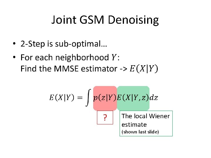
Joint GSM Denoising • ? The local Wiener estimate (shown last slide)

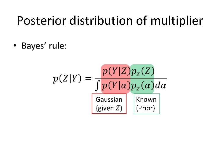
Posterior distribution of multiplier • Known (Prior)

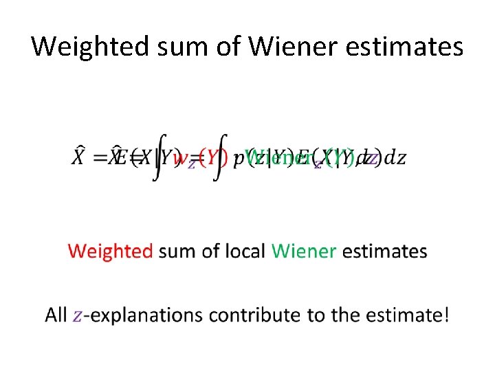
Weighted sum of Wiener estimates •

BLS-GSM-Wavelet Denoising Local neighborhood Decompose to Wavelet sub-bands “sophisticated” Wiener Filter GSM Local neighborhood “sophisticated” Wiener Filter GSM . . . Local neighborhood “sophisticated” Wiener Filter GSM “Clean” Wavelet sub -bands

State of the art Methods BLSGSM BM 3 D NLM Spatial Methods Transform Methods

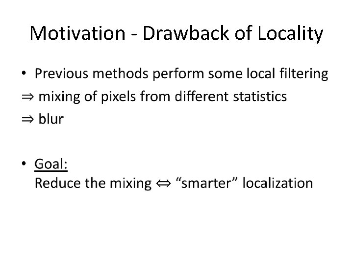
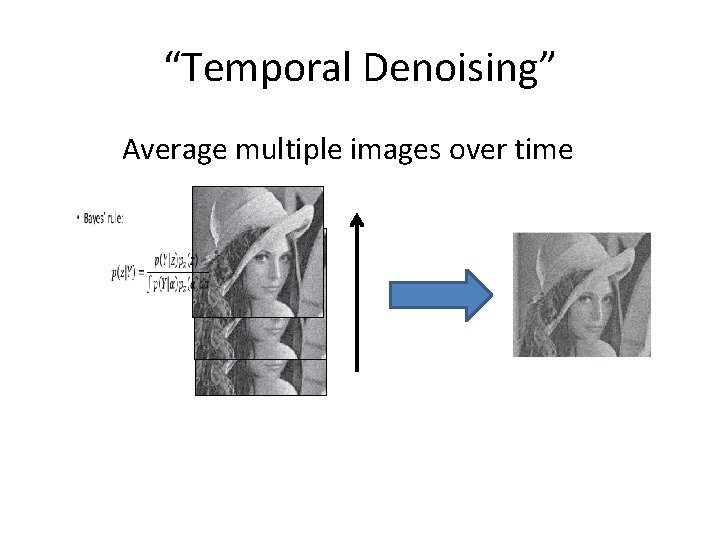
Motivation - Drawback of Locality •

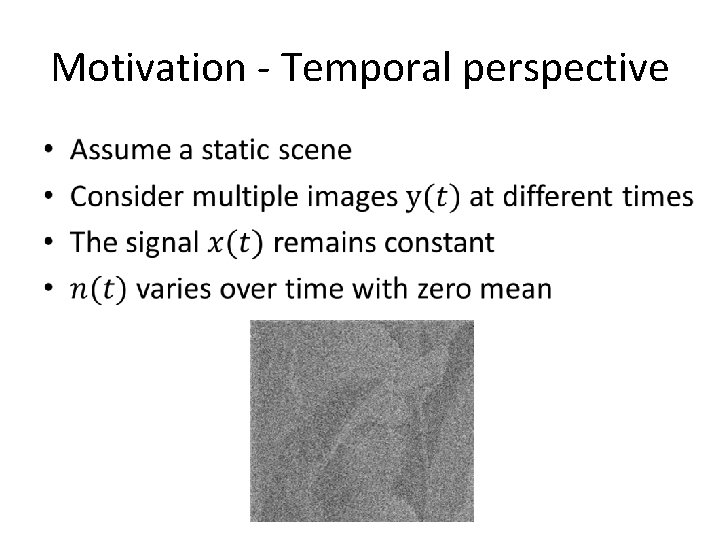
Motivation - Temporal perspective •

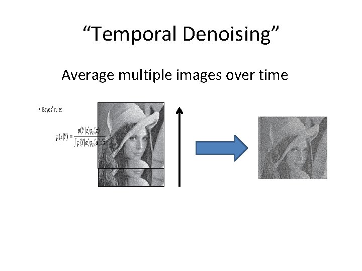
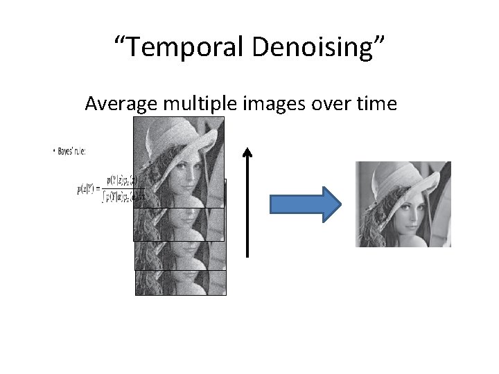
“Temporal Denoising” Average multiple images over time

“Temporal Denoising” Average multiple images over time

“Temporal Denoising” Average multiple images over time

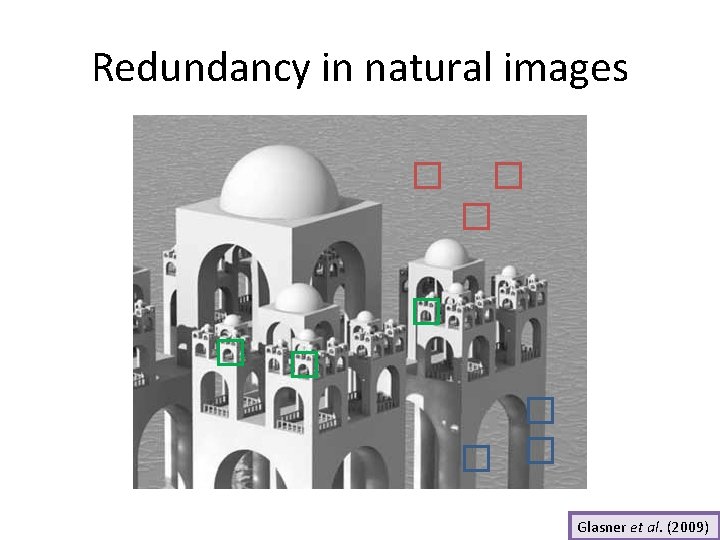
Redundancy in natural images Glasner et al. (2009)

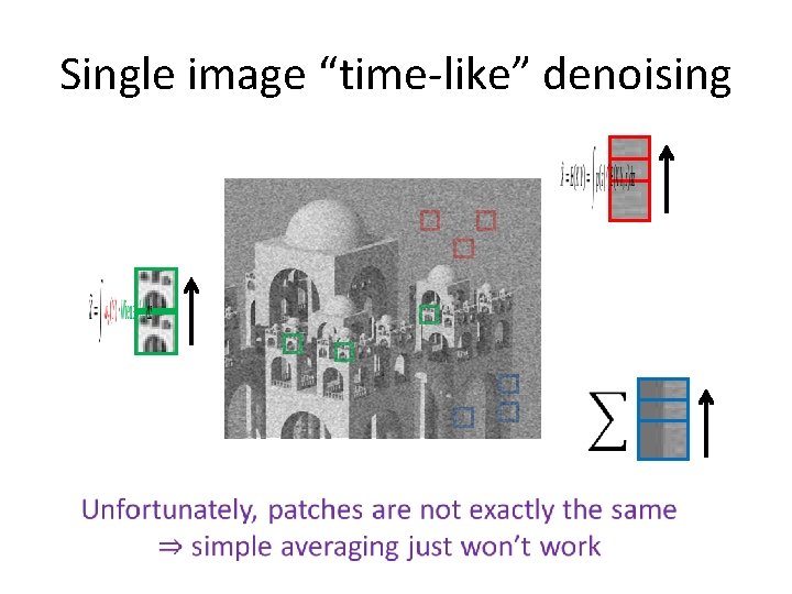
Single image “time-like” denoising

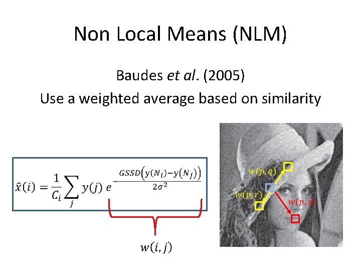
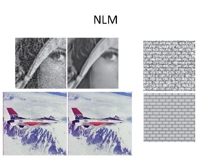
Non Local Means (NLM) Baudes et al. (2005) Use a weighted average based on similarity

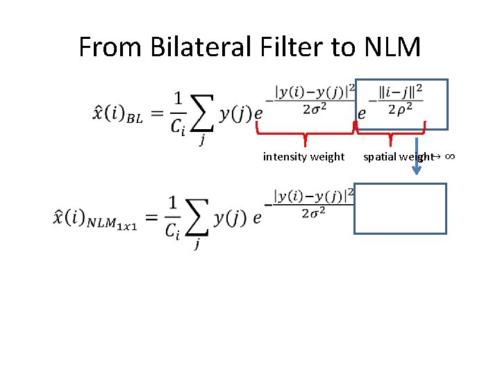
From Bilateral Filter to NLM intensity weight spatial weight

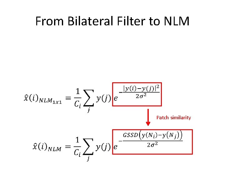
From Bilateral Filter to NLM Patch similarity

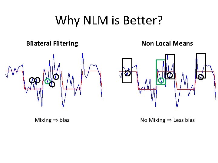
Why NLM is Better? Non Local Means Bilateral Filtering

Performance Evaluation Method Noise Gaussian Smoothing Anisotropic Filtering Bilateral Filtering NLM Windowed Weiner Hard WT Soft WT Buades et al. (2005)

What’s Next? •

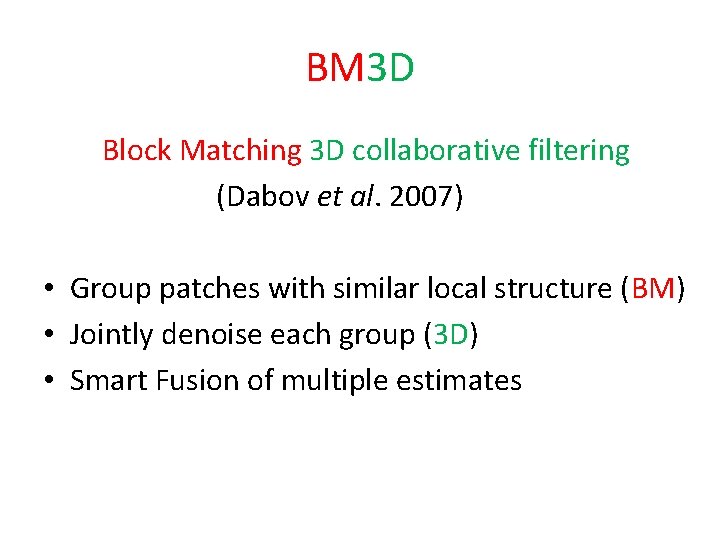
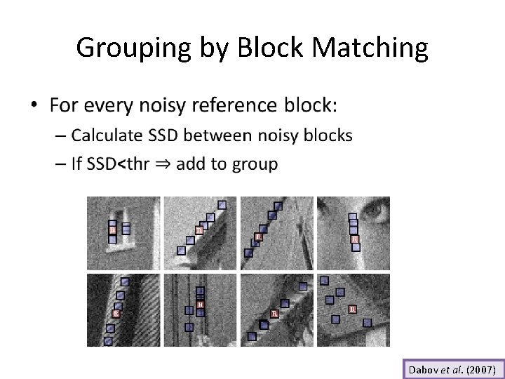
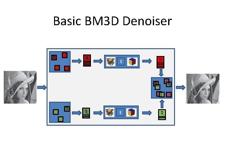
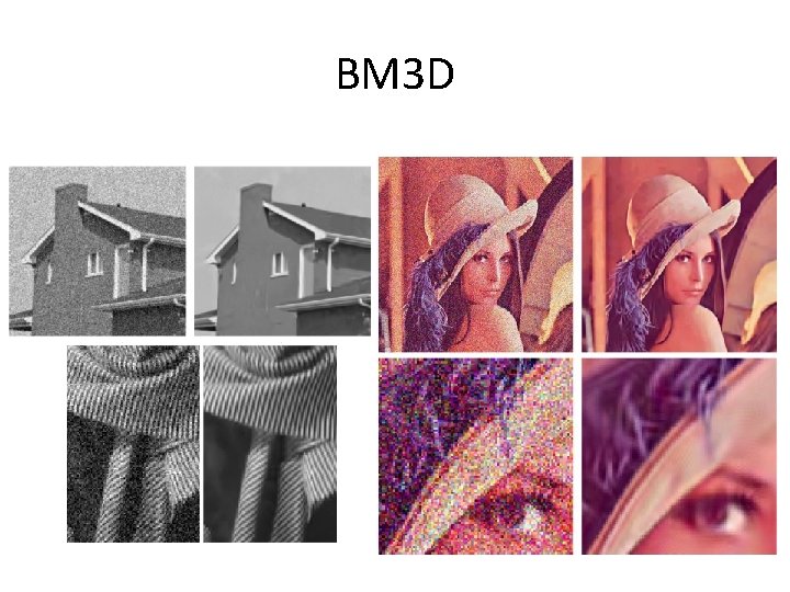
BM 3 D Block Matching 3 D collaborative filtering (Dabov et al. 2007) • Group patches with similar local structure (BM) • Jointly denoise each group (3 D) • Smart Fusion of multiple estimates

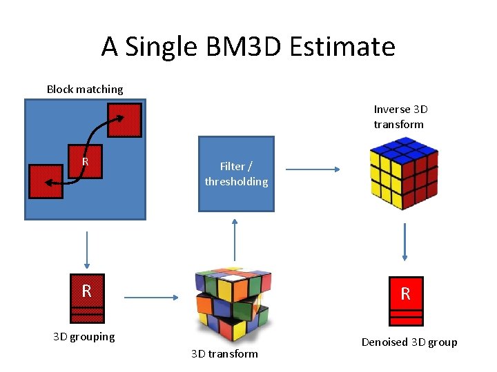
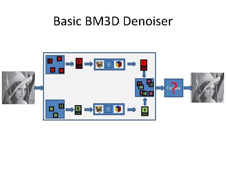
A Single BM 3 D Estimate Block matching Inverse 3 D transform R Filter / thresholding R R 3 D grouping Denoised 3 D group 3 D transform

Grouping by Block Matching • Dabov et al. (2007)

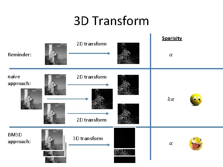
3 D Transform 2 D transform Reminder: naive approach: Sparisity 2 D transform BM 3 D approach: 3 D transform

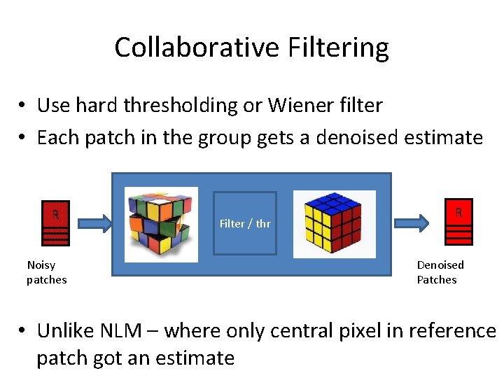
Collaborative Filtering • Use hard thresholding or Wiener filter • Each patch in the group gets a denoised estimate R Noisy patches Filter / thr R Denoised Patches • Unlike NLM – where only central pixel in reference patch got an estimate

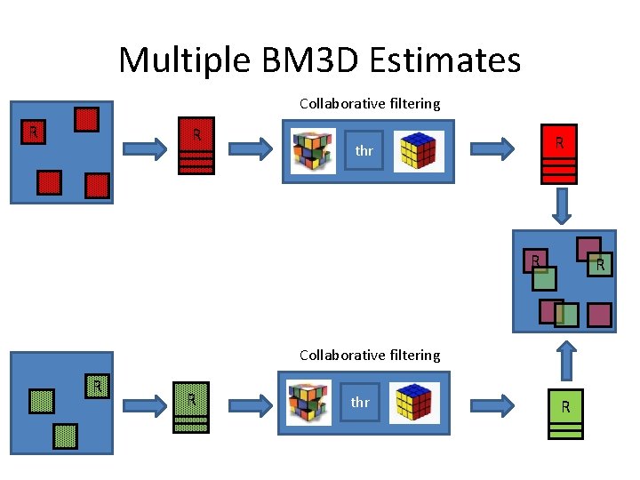
Multiple BM 3 D Estimates Collaborative filtering R R R thr R R Collaborative filtering R R thr R

Basic BM 3 D Denoiser R R R t R R ? Fusion

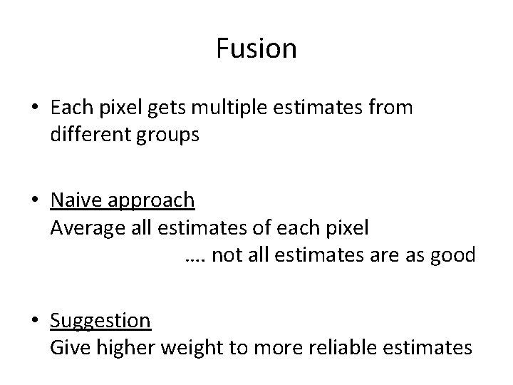
Fusion • Each pixel gets multiple estimates from different groups • Naive approach Average all estimates of each pixel …. not all estimates are as good • Suggestion Give higher weight to more reliable estimates

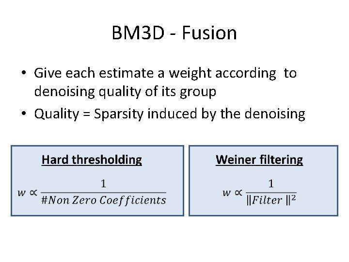
BM 3 D - Fusion • Give each estimate a weight according to denoising quality of its group • Quality = Sparsity induced by the denoising

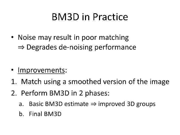
BM 3 D in Practice •

Basic BM 3 D Denoiser R R R t R R

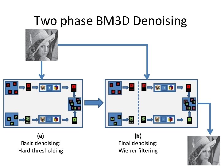
Two phase BM 3 D Denoising R R R t (a) Basic denoising: Hard thresholding R R t R R R (b) Final denoising: Wiener filtering t R R

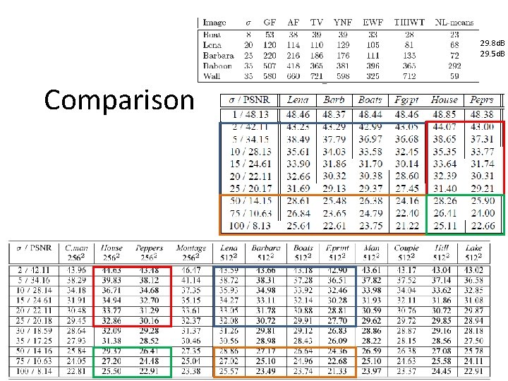
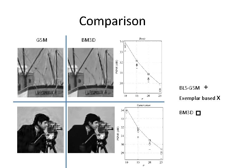
Results and Comparison • Comparison: – Different levels of noise – Different sets of images • Evaluation methods: – MSE/PSNR – Visual comparison to noisy and/or original images

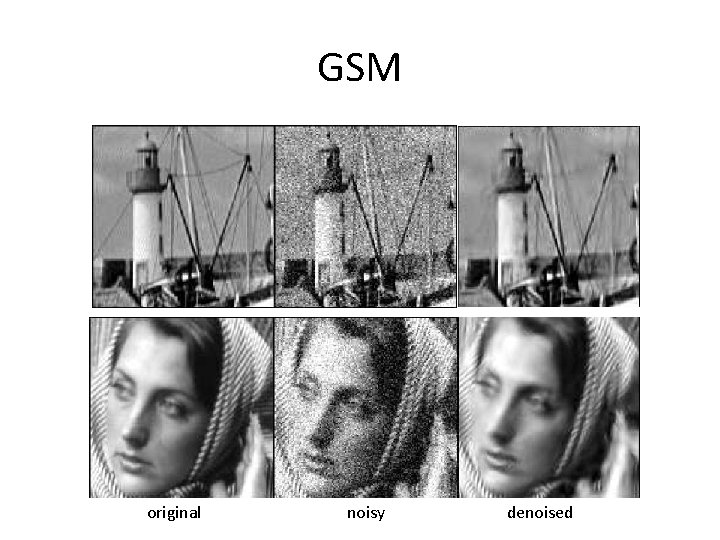
GSM original noisy denoised

NLM

BM 3 D

29. 8 d. B 29. 5 d. B Comparison

Comparison GSM BM 3 D BLS-GSM + Exemplar based x BM 3 D

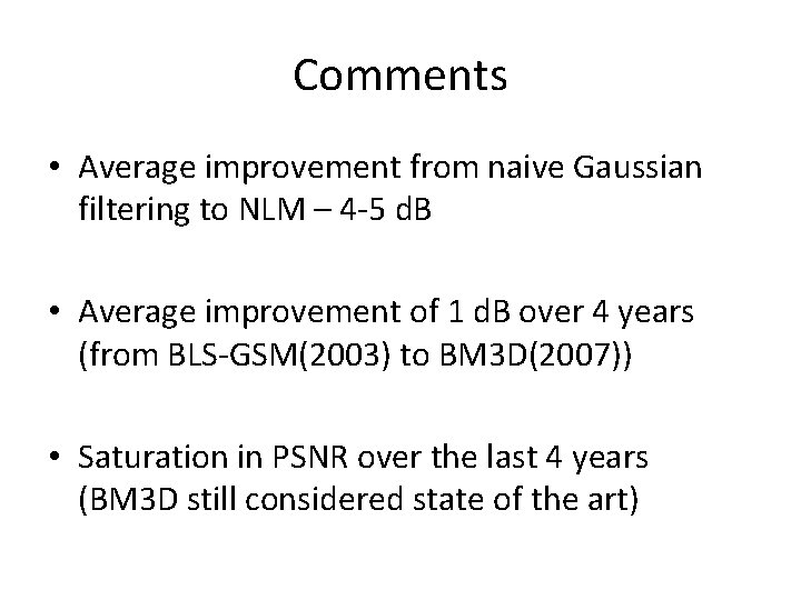
Comments • Average improvement from naive Gaussian filtering to NLM – 4 -5 d. B • Average improvement of 1 d. B over 4 years (from BLS-GSM(2003) to BM 3 D(2007)) • Saturation in PSNR over the last 4 years (BM 3 D still considered state of the art)