
DeepTime Data Infrastructure A DCO Legacy Program Robert
Deep-Time Data Infrastructure: A DCO Legacy Program Robert M. Hazen—Geophysical Lab, Carnegie Institution DCO Data Science Day—RPI—June 5, 2014
Conclusions Vast, largely untapped, data resources inform our view of Earth’s dynamic history over 4. 5 billion years. Combining those deep-time data resources into a single infrastructure represents an opportunity for accelerated “abductive” discovery.
Deep-Time Data Collaborators Carnegie Institution Robert Hazen Xiaoming Liu Anat Shahar Rutgers Paul Falkowski RPI Peter Fox Univ. of Arizona Robert Downs Mihei Ducea Grethe Hystad Barbara Lafuente Hexiong Yang Alex Pires Joaquin Ruiz Joshua Golden Melissa Mc. Millan Shaunna Morrison Johns Hopkins Univ. Cal. Tech Dimitri Sverjensky Ralph Milliken Charlene Estrada Univ. of Maine John Ferry Edward Grew Namhey Lee Smithsonian Inst. Harvard University Timothy Mc. Coy Andrew Knoll Univ. of Manitoba Indiana University Andrey Bekker David Bish MINDAT. ORG Univ. of Michigan Jolyon Ralph Rodney Ewing Colorado State Holly Stein Univ. of Maryland Aaron Zimmerman James Farquhar Univ. of Tennessee John Nance Linda Kah Univ. of Wisconsin Univ College London John Valley Geol. Survey Canada Dominic Papineau George Mason Univ. Wouter Bleeker Stephen Elmore
Deep-Time Data Resources Mineralogy and petrology data: Mineral species and assemblages Compositions (including isotopes) Age (ages) Geographic location; tectonic setting Crystal size; morphology; twinning Solid and fluid inclusions; defects; Magnetic domains; zoning; exsolution Surface properties; grain boundaries
Deep-Time Data Resources Mineralogy and petrology data Paleobiology data Fossil species and assemblages Age Biominerals; isotopic composition Molecular biomarkers Host lithology Geological/tectonic context
Deep-Time Data Resources Mineralogy and petrology data Paleobiology data Proteomics data Enzyme structure and function Age (from phylogenetics) Active site composition Microbial context
Deep-Time Data Resources Mineralogy and petrology data Paleobiology data Proteomics data Geochemistry data and modeling Thermochemical data Equilibrium and reaction path models
Deep-Time Data Resources Mineralogy and petrology data Paleobiology data Proteomics data Geochemistry data and modeling Paleotectonic & Paleomagnetic Data Age
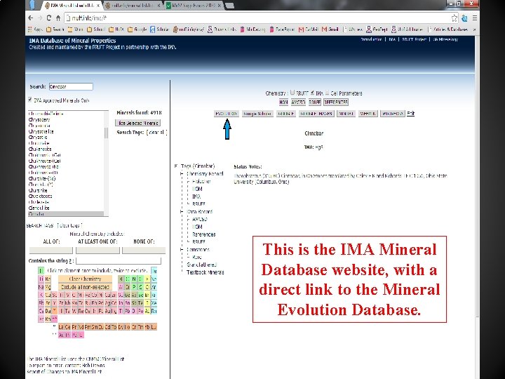
This is the IMA Mineral Database website, with a direct link to the Mineral Evolution Database.
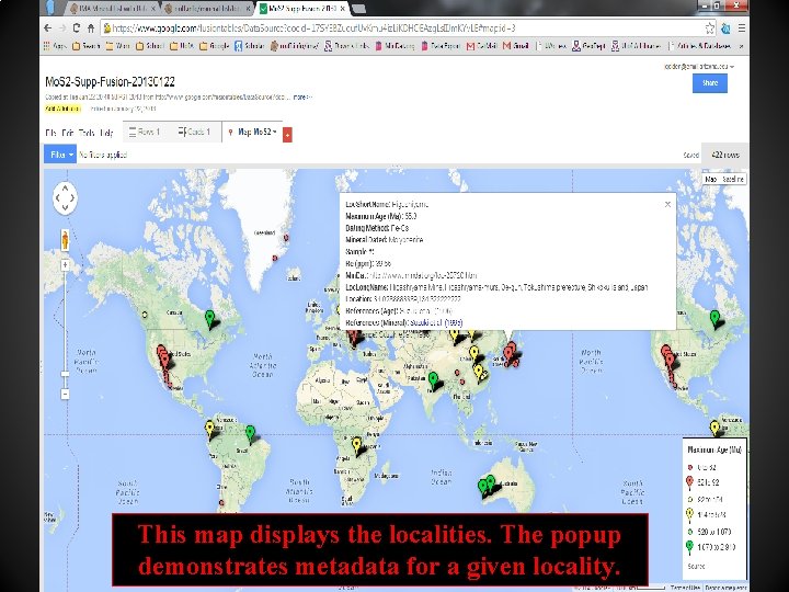
This map displays the localities. The popup demonstrates metadata for a given locality.
The Potential of Deep-Time Data The Premise: Rocks, minerals, fossils, and life’s biochemistry hold clues to significant changes in Earth’s near-surface environment through 4. 5 billion years of history.
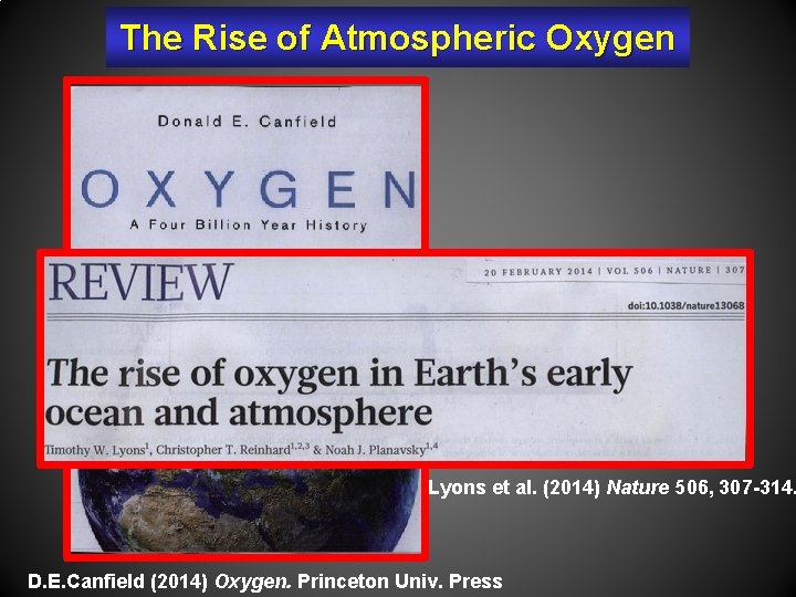
The Rise of Atmospheric Oxygen Lyons et al. (2014) Nature 506, 307 -314. D. E. Canfield (2014) Oxygen. Princeton Univ. Press
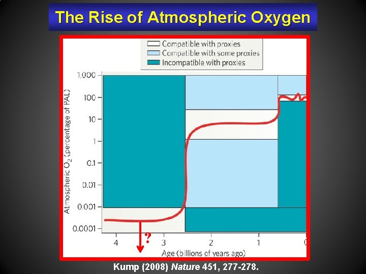
The Rise of Atmospheric Oxygen ? Kump (2008) Nature 451, 277 -278.
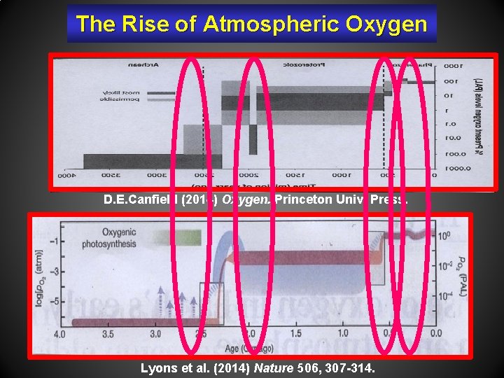
The Rise of Atmospheric Oxygen D. E. Canfield (2014) Oxygen. Princeton Univ. Press. Lyons et al. (2014) Nature 506, 307 -314.
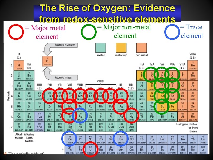
The Rise of Oxygen: Evidence from redox-sensitive elements = Major metal element = Major non-metal element = Trace element
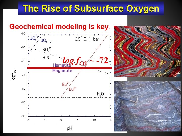
The Rise of Subsurface Oxygen Geochemical modeling is key. log f. O 2 ~ -72
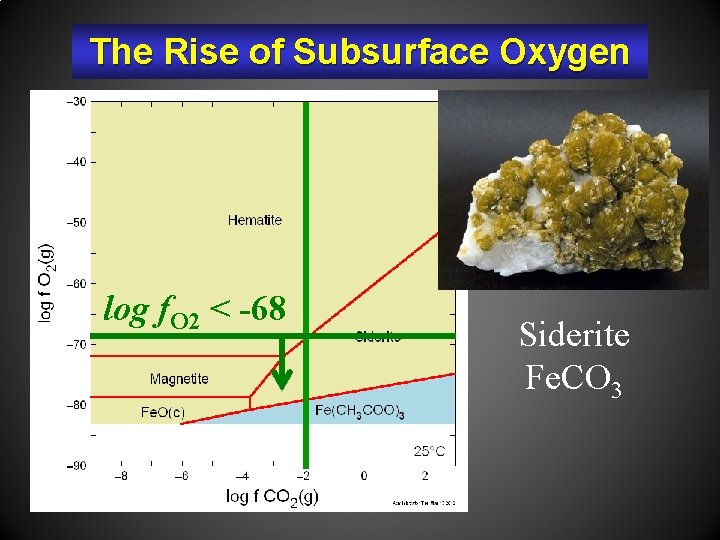
The Rise of Subsurface Oxygen log f. O 2 < -68 Siderite Fe. CO 3
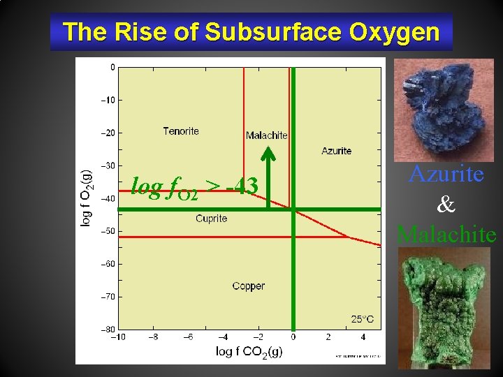
The Rise of Subsurface Oxygen log f. O 2 > -43 Azurite & Malachite
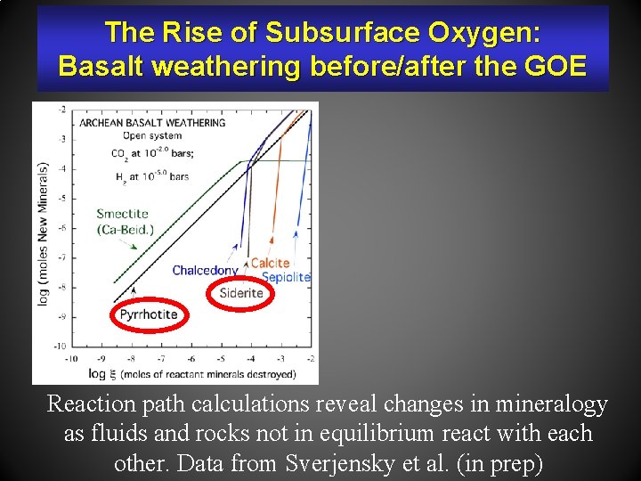
The Rise of Subsurface Oxygen: Basalt weathering before/after the GOE Reaction path calculations reveal changes in mineralogy as fluids and rocks not in equilibrium react with each other. Data from Sverjensky et al. (in prep)
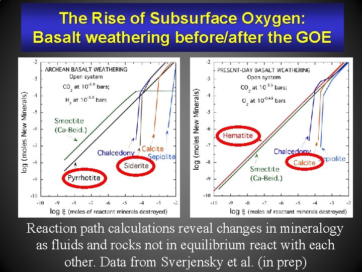
The Rise of Subsurface Oxygen: Basalt weathering before/after the GOE Reaction path calculations reveal changes in mineralogy as fluids and rocks not in equilibrium react with each other. Data from Sverjensky et al. (in prep)
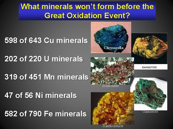
What minerals won’t form before the Great Oxidation Event? 598 of 643 Cu minerals Chrysocolla 202 of 220 U minerals 319 of 451 Mn minerals Piemontite 47 of 56 Ni minerals 582 of 790 Fe minerals Garnierite Xanthoxenite
Co-evolution of the geosphere and biosphere Biologically mediated changes in Earth’s atmospheric composition at ~2. 4 to 2. 2 Ga represent the single most significant factor in Earth’s mineralogical diversity.
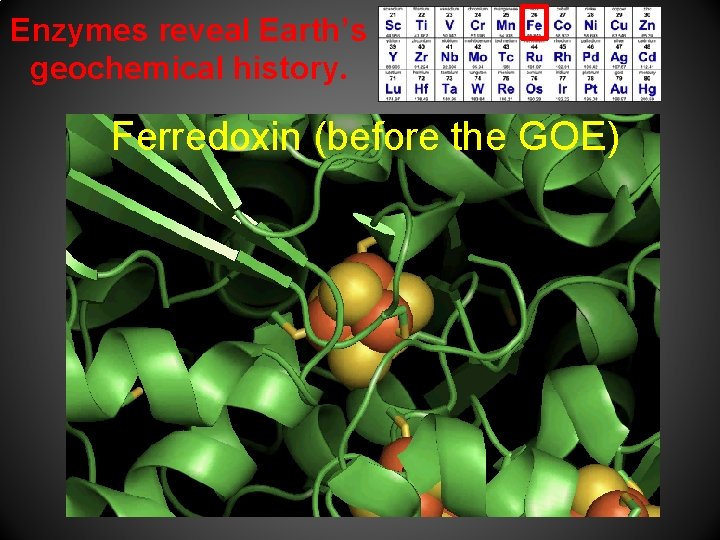
Enzymes reveal Earth’s geochemical history. Ferredoxin (before the GOE)
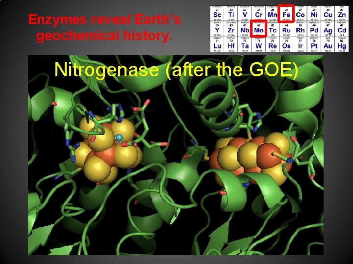
Enzymes reveal Earth’s geochemical history. Nitrogenase (after the GOE)
The Rise of Subsurface Oxygen
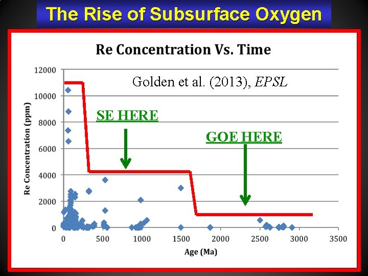
The Rise of Subsurface Oxygen Golden et al. (2013), EPSL SE HERE GOE HERE
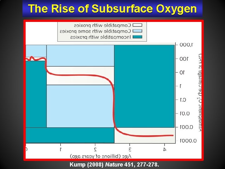
The Rise of Subsurface Oxygen Kump (2008) Nature 451, 277 -278.
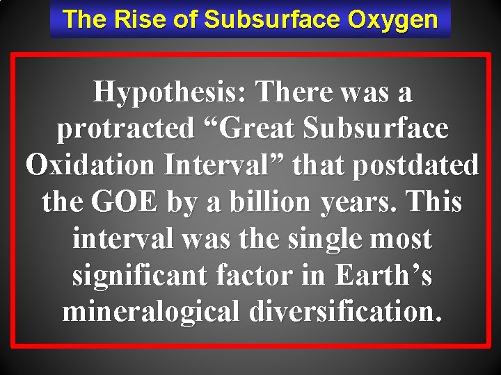
The Rise of Subsurface Oxygen Hypothesis: There was a protracted “Great Subsurface Oxidation Interval” that postdated the GOE by a billion years. This interval was the single most significant factor in Earth’s mineralogical diversification.
Data-Driven Discovery Most of what scientists do most of the time is start with a known phenomenon, and then collect relevant data and develop explanatory hypotheses.
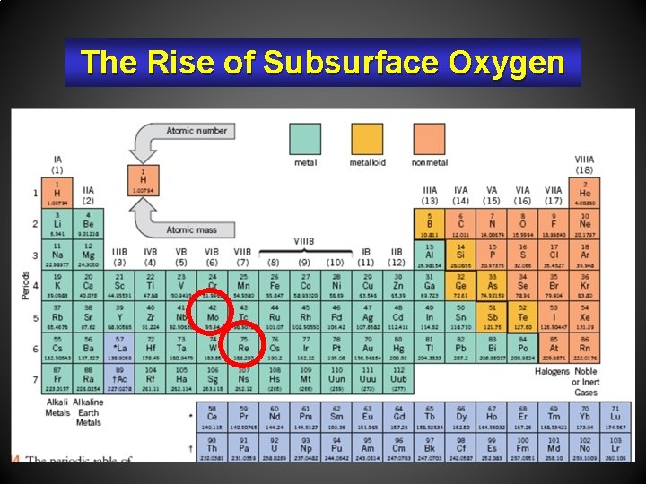
Deduction Earth’s atmospheric oxidation influenced the partitioning of redox-sensitive elements. Mo, Re, Ni, and Co are redox-sensitive elements. Therefore, we deduce that atmospheric oxidation influenced the partitioning of Mo, Re, Ni, and Co.
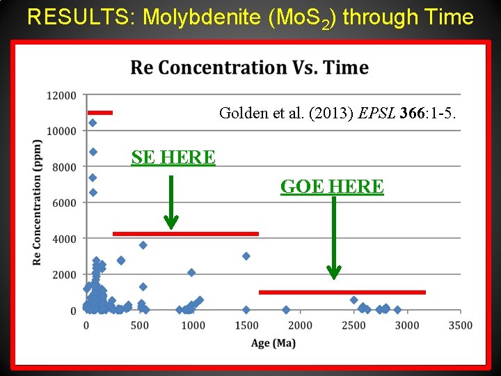
RESULTS: Molybdenite (Mo. S 2) through Time Golden et al. (2013) EPSL 366: 1 -5. SE HERE GOE HERE
RESULTS: Cu/Ni in carbonates vs. time Xiaoming Liu et al. (2013) SE HERE GOE HERE
Induction Each of the last 5 supercontinent cycles led to episodes of enhanced mineralization during intervals of continental convergence. Mo, Be, B, and Hg are mineral-forming elements. Therefore, we predict by induction that Mo, Be, B, and Hg minerals will display enhanced mineralization during intervals of continental convergence.
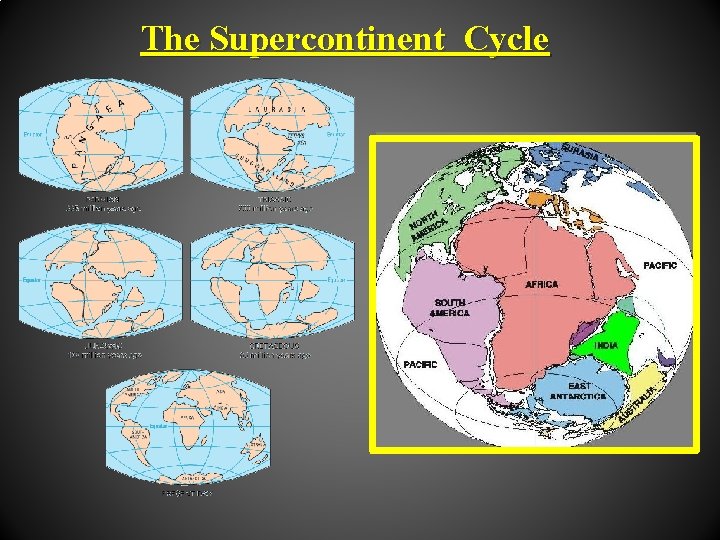
The Supercontinent Cycle
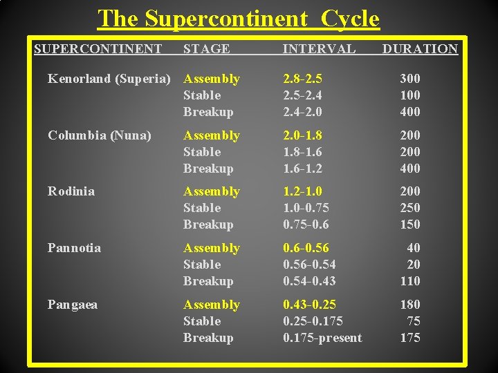
The Supercontinent Cycle SUPERCONTINENT STAGE INTERVAL DURATION Kenorland (Superia) Assembly Stable Breakup 2. 8 -2. 5 -2. 4 -2. 0 300 100 400 Columbia (Nuna) Assembly Stable Breakup 2. 0 -1. 8 -1. 6 -1. 2 200 400 Rodinia Assembly Stable Breakup 1. 2 -1. 0 -0. 75 -0. 6 200 250 150 Pannotia Assembly Stable Breakup 0. 6 -0. 56 -0. 54 -0. 43 40 20 110 Pangaea Assembly Stable Breakup 0. 43 -0. 25 -0. 175 -present 180 75 175
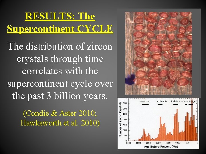
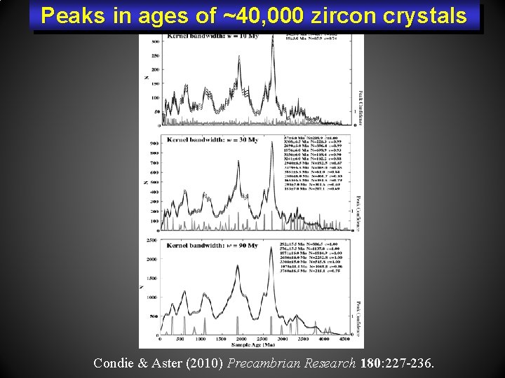
RESULTS: The Supercontinent CYCLE The distribution of zircon crystals through time correlates with the supercontinent cycle over the past 3 billion years. (Condie & Aster 2010; Hawksworth et al. 2010)
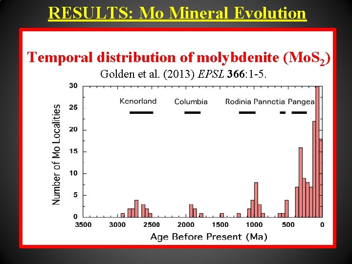
RESULTS: Mo Mineral Evolution Temporal distribution of molybdenite (Mo. S 2) Golden et al. (2013) EPSL 366: 1 -5.
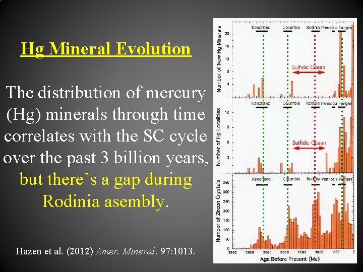
Hg Mineral Evolution The distribution of mercury (Hg) minerals through time correlates with the SC cycle over the past 3 billion years, but there’s a gap during Rodinia asembly. Hazen et al. (2012) Amer. Mineral. 97: 1013.
Abduction is a form of logical inference that goes from reliable data (i. e. , observations), to a hypothesis that seeks to explain those data. (Paraphrased from Wikipedia)
Abduction Observations lead to new hypotheses. We have vast amounts of data on mineral species, compositions, isotopes, petrologic context, thermochemical parameters, tectonic settings, and the co-evolving biosphere through deep time. Previously unrecognized patterns and correlations will emerge from the integration and evaluation of those data.
Data-Driven Discovery THE CHALLENGE: Recognizing statistically meaningful patterns in large data resources: 1. Correlations among many variables
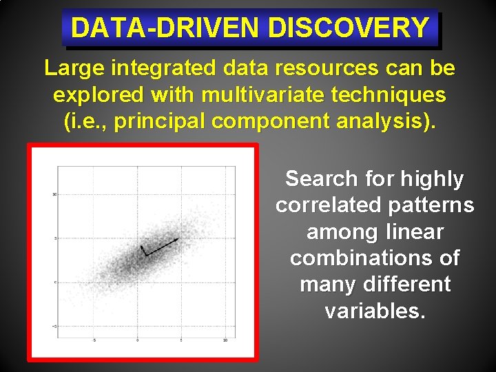
DATA-DRIVEN DISCOVERY Large integrated data resources can be explored with multivariate techniques (i. e. , principal component analysis). Search for highly correlated patterns among linear combinations of many different variables.
Data-Driven Discovery THE CHALLENGE: Recognizing statistically meaningful patterns in large data resources: 2. Meaningful trends in data vs. time
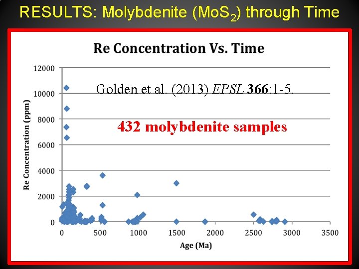
RESULTS: Molybdenite (Mo. S 2) through Time Golden et al. (2013) EPSL 366: 1 -5. 432 molybdenite samples
Are these trends statistically significant? • Analyze equal sized bins. • Apply statistical tests: linear regression of log Re content vs. time. (Montgomery et al. 2006)
Data-Driven Discovery THE CHALLENGE: Recognizing statistically meaningful patterns in large data resources: 3. Peak-to-noise problem
Peaks in ages of ~40, 000 zircon crystals Condie & Aster (2010) Precambrian Research 180: 227 -236.
Monte Carlo Mean Kernal Density Analysis Condie & Aster (2010) Precambrian Research 180: 227 -236.
Data-Driven Discovery THE CHALLENGE: Recognizing statistically meaningful patterns in large data resources: 4. Visualization opportunities
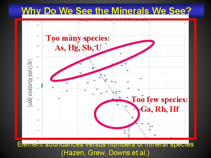
Why Do We See the Minerals We See? Too many species: As, Hg, Sb, U Too few species: Ga, Rb, Hf Element abundances versus numbers of mineral species (Hazen, Grew, Downs et al. )
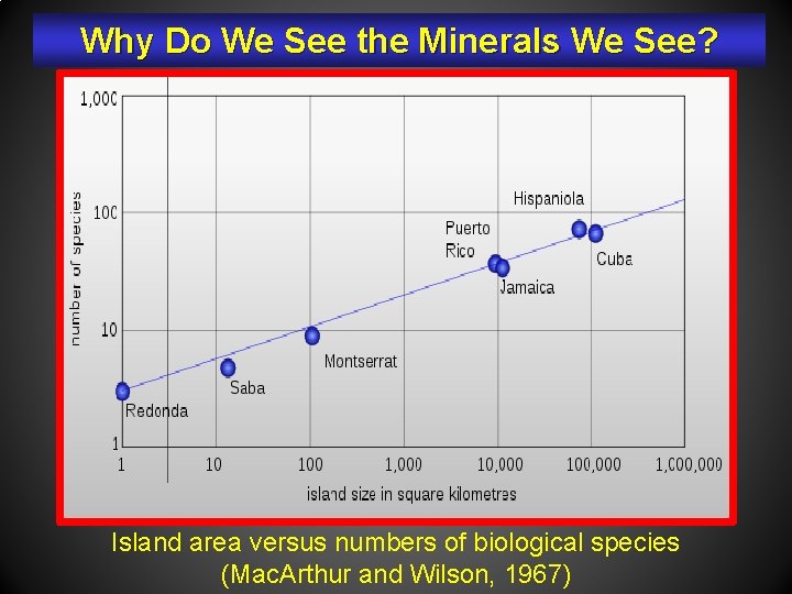
Why Do We See the Minerals We See? Island area versus numbers of biological species (Mac. Arthur and Wilson, 1967)
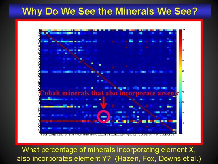
Why Do We See the Minerals We See? Cobalt minerals that also incorporate arsenic What percentage of minerals incorporating element X, also incorporates element Y? (Hazen, Fox, Downs et al. )
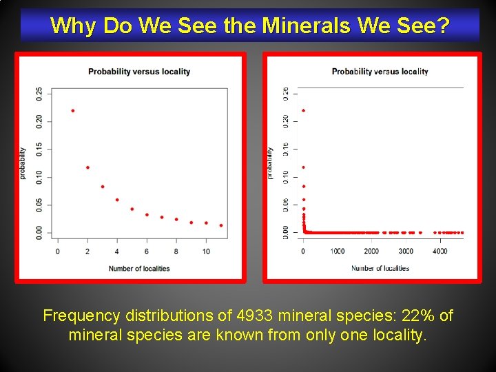
Why Do We See the Minerals We See? Frequency distributions of 4933 mineral species: 22% of mineral species are known from only one locality.
Why Do We See the Minerals We See? Frequency distributions of 4933 mineral species: 22% of mineral species are known from only one locality. Therefore: (1) Numerous additional minerals exist on Earth but as yet remain undescribed. (2) Numerous other plausible minerals do not now exist on Earth, but might have in the past, or might occur on other Earth-like planets. (3) If we “played the tape over again, ” then the first 4933 minerals to be found would likely differ by ~1000 mineral species.
Conclusions Vast, largely untapped, data resources inform our view of Earth’s dynamic history over 4. 5 billion years. Combining those deep-time data resources into a single infrastructure represents an opportunity for accelerated “abductive” discovery.
Data-Driven Discovery CONCLUSIONS We are poised to make fundamental discoveries about our planetary home through development, integration, and exploration of deep-time data resources.
Please join this effort: • Archive your data • Release “dark data” • Help us build this resource
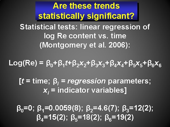
Are these trends statistically significant? Statistical tests: linear regression of log Re content vs. time (Montgomery et al. 2006): Log(Re) = β 0+β 1 t+β 2 x 2+β 3 x 3+β 4 x 4+β 5 x 5+β 6 x 6 [t = time; βi = regression parameters; xi = indicator variables] β 0=0; β 1=0. 0059(8); β 2=4. 6(7); β 3=12(2); β 4=15(2); β 5=18(2); β 6=19(2)
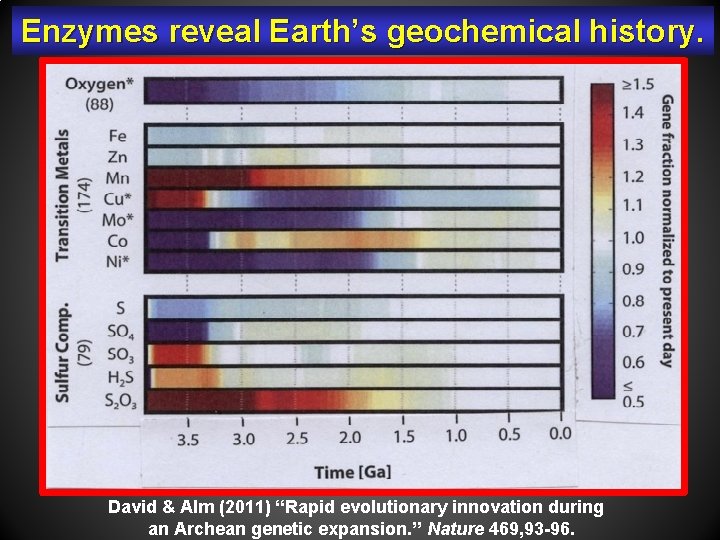
Enzymes reveal Earth’s geochemical history. David & Alm (2011) “Rapid evolutionary innovation during an Archean genetic expansion. ” Nature 469, 93 -96.
- Slides: 59