15 853 Algorithms in the Real World Computational

15 -853: Algorithms in the Real World Computational Biology II – Sequence Alignment – Database searches 15 -853 Page 1

Extending LCS for Biology The LCS/Edit distance problem is not a “practical” model for comparing DNA or proteins. Why? Good example of the simple model failing. 15 -853 Page 2

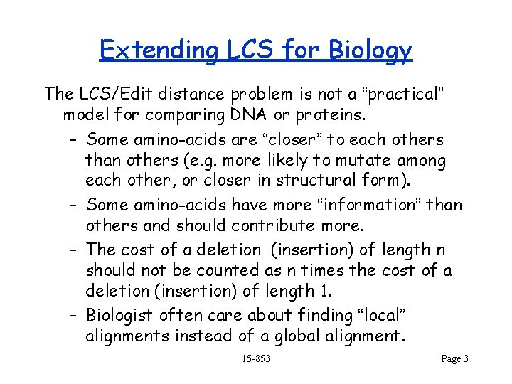
Extending LCS for Biology The LCS/Edit distance problem is not a “practical” model for comparing DNA or proteins. – Some amino-acids are “closer” to each others than others (e. g. more likely to mutate among each other, or closer in structural form). – Some amino-acids have more “information” than others and should contribute more. – The cost of a deletion (insertion) of length n should not be counted as n times the cost of a deletion (insertion) of length 1. – Biologist often care about finding “local” alignments instead of a global alignment. 15 -853 Page 3

What we will talk about today Extensions • Sequence Alignment: a generalization of LCS to account for the closeness of different elements • Gap Models: More sophisticated models for accounting for the cost of adjacent insertions or deletions • Local Alignment: Finding parts of one sequence in parts of another sequence. Applications • FASTA and BLAST: The most common sequence matching tools used in Molecular Biology. 15 -853 Page 4

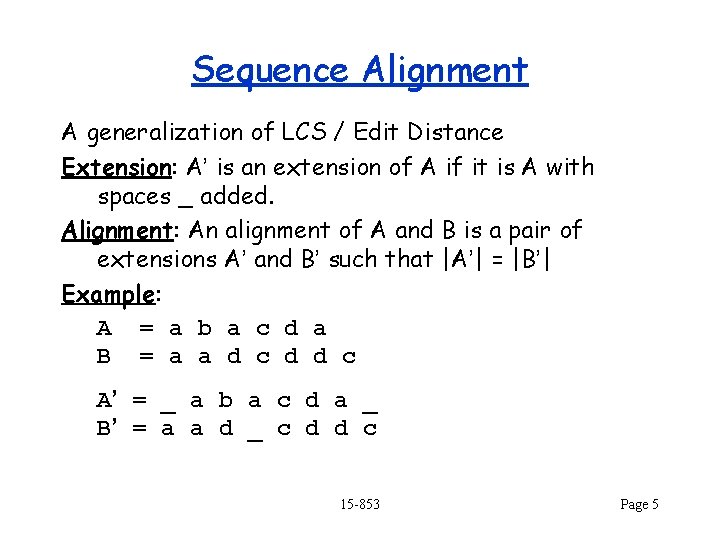
Sequence Alignment A generalization of LCS / Edit Distance Extension: A’ is an extension of A if it is A with spaces _ added. Alignment: An alignment of A and B is a pair of extensions A’ and B’ such that |A’| = |B’| Example: A = a b a c d a B = a a d c d d c A’ = _ a b a c d a _ B’ = a a d _ c d d c 15 -853 Page 5

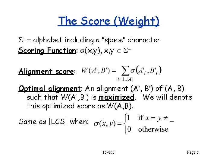
The Score (Weight) S+ = alphabet including a “space” character Scoring Function: s(x, y), x, y S+ Alignment score: Optimal alignment: An alignment (A’, B’) of (A, B) such that W(A’, B’) is maximized. We will denote this optimized score as W(A, B). Same as |LCS| when: 15 -853 Page 6

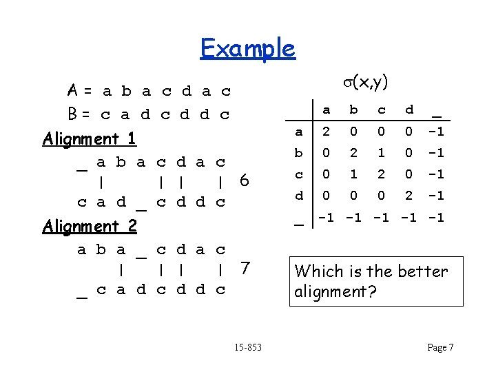
Example s(x, y) A= a b a c d a c B= c a d c d d c Alignment 1 _ a b a c d a c | | 6 c a d _ c d d c Alignment 2 a b a _ c d a c | | 7 _ c a d c d d c 15 -853 a b c d _ a 2 0 0 0 -1 b 0 2 1 0 -1 c 0 1 2 0 -1 d 0 0 0 2 -1 _ -1 -1 -1 Which is the better alignment? Page 7

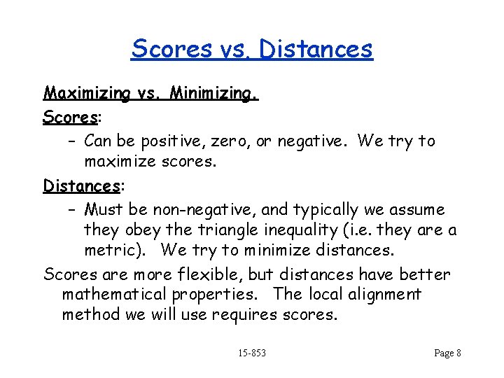
Scores vs. Distances Maximizing vs. Minimizing. Scores: – Can be positive, zero, or negative. We try to maximize scores. Distances: – Must be non-negative, and typically we assume they obey the triangle inequality (i. e. they are a metric). We try to minimize distances. Scores are more flexible, but distances have better mathematical properties. The local alignment method we will use requires scores. 15 -853 Page 8

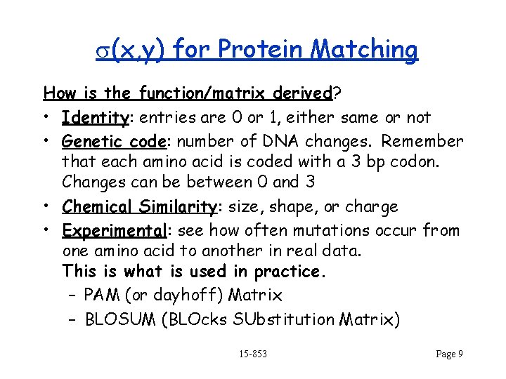
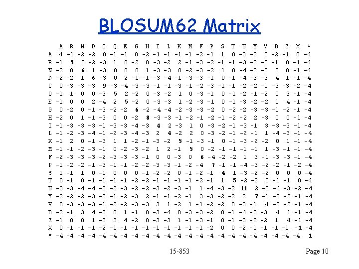
s(x, y) for Protein Matching How is the function/matrix derived? • Identity: entries are 0 or 1, either same or not • Genetic code: number of DNA changes. Remember that each amino acid is coded with a 3 bp codon. Changes can be between 0 and 3 • Chemical Similarity: size, shape, or charge • Experimental: see how often mutations occur from one amino acid to another in real data. This is what is used in practice. – PAM (or dayhoff) Matrix – BLOSUM (BLOcks SUbstitution Matrix) 15 -853 Page 9

BLOSUM 62 Matrix A R N D C Q E G H I L K M F P S T W Y V B Z X * A 4 -1 -2 -2 0 -1 -1 0 -2 -1 -1 -2 -1 1 0 -3 -2 0 -2 -1 0 -4 R -1 5 0 -2 -3 1 0 -2 0 -3 -2 2 -1 -3 -2 -1 -1 -3 -2 -3 -1 0 -1 -4 N -2 0 6 1 -3 0 0 0 1 -3 -3 0 -2 -3 -2 1 0 -4 -2 -3 3 0 -1 -4 D -2 -2 1 6 -3 0 2 -1 -1 -3 -4 -1 -3 -3 -1 0 -1 -4 -3 -3 4 1 -1 -4 C 0 -3 -3 -3 9 -3 -4 -3 -3 -1 -1 -3 -1 -2 -3 -1 -1 -2 -2 -1 -3 -3 -2 -4 Q -1 1 0 0 -3 5 2 -2 0 -3 -2 1 0 -3 -1 0 -1 -2 0 3 -1 -4 E -1 0 0 2 -4 2 5 -2 0 -3 -3 1 -2 -3 -1 0 -1 -3 -2 -2 1 4 -1 -4 G 0 -2 0 -1 -3 -2 -2 6 -2 -4 -4 -2 -3 -3 -2 0 -2 -2 -3 -3 -1 -2 -1 -4 H -2 0 1 -1 -3 0 0 -2 8 -3 -3 -1 -2 -2 2 -3 0 0 -1 -4 I -1 -3 -3 -3 -1 -3 -3 -4 -3 4 2 -3 1 0 -3 -2 -1 -3 -1 3 -3 -3 -1 -4 L -1 -2 -3 -4 -3 2 4 -2 2 0 -3 -2 -1 1 -4 -3 -1 -4 K -1 2 0 -1 -3 1 1 -2 -1 -3 -2 5 -1 -3 -1 0 -1 -3 -2 -2 0 1 -1 -4 M -1 -1 -2 -3 -1 0 -2 -3 -2 1 2 -1 5 0 -2 -1 -1 1 -3 -1 -1 -4 15 -853 F -2 -3 -3 -3 -1 0 0 -3 0 6 -4 -2 -2 1 3 -1 -3 -3 -1 -4 P -1 -2 -2 -1 -3 -1 -1 -2 -2 -3 -3 -1 -2 -4 7 -1 -1 -4 -3 -2 -2 -1 -2 -4 S 1 -1 1 0 -1 0 0 0 -1 -2 -2 0 -1 -2 -1 4 1 -3 -2 -2 0 0 0 -4 T 0 -1 -1 -2 -2 -1 -1 -2 -1 1 5 -2 -2 0 -1 -1 0 -4 W -3 -3 -4 -4 -2 -2 -3 -1 1 -4 -3 -2 11 2 -3 -4 -3 -2 -4 Y -2 -2 -2 -3 -2 -1 -2 -3 2 -1 -1 -2 -1 3 -3 -2 -2 2 7 -1 -3 -2 -1 -4 V 0 -3 -3 -3 -1 -2 -2 -3 -3 3 1 -2 1 -1 -2 -2 0 -3 -1 4 -3 -2 -1 -4 B -2 -1 3 4 -3 0 1 -1 0 -3 -4 0 -3 -3 -2 0 -1 -4 -3 -3 4 1 -1 -4 Z -1 0 0 1 -3 3 4 -2 0 -3 -3 1 -1 -3 -1 0 -1 -3 -2 -2 1 4 -1 -4 X 0 -1 -1 -1 -2 -1 -1 -1 -2 0 0 -2 -1 -1 -1 -4 * -4 -4 -4 -4 -4 -4 1 Page 10

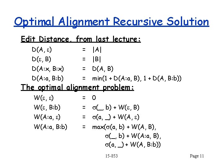
Optimal Alignment Recursive Solution Edit Distance, from last lecture: D(A, e) = |A| D(e, B) = |B| D(A: x, B: x) = D(A, B) D(A: a, B: b) = min(1 + D(A: a, B), 1 + D(A, B: b)) W(e, e) = 0 W(e, B: b) = s(_, b) + W(e, B) W(A: a, e) = s(a, _) + W(A, e) W(A: a, B: b) = max(s(a, b) + W(A, B), s(_, b) + W(A: a, B), s(a, _) + W(A, B: b)) The optimal alignment problem: 15 -853 Page 11

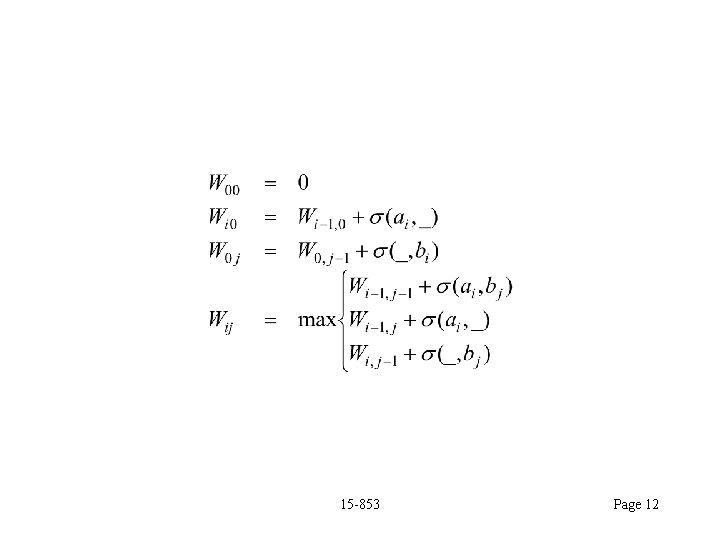
15 -853 Page 12

Dynamic programming for i = 1 M[i, 1] for j = 1 M[1, j] to n = s(A[i], _ ) to m = s(_ , B[i]); for i = 1 to n for j = 1 to m M[i, j] = max 3(s(A[i], B[j]) + M[i-1, j-1], s(A[i], _ ) + M[i-1, j], s( _ , B[j]) + M[i , j-1]); 15 -853 Page 13

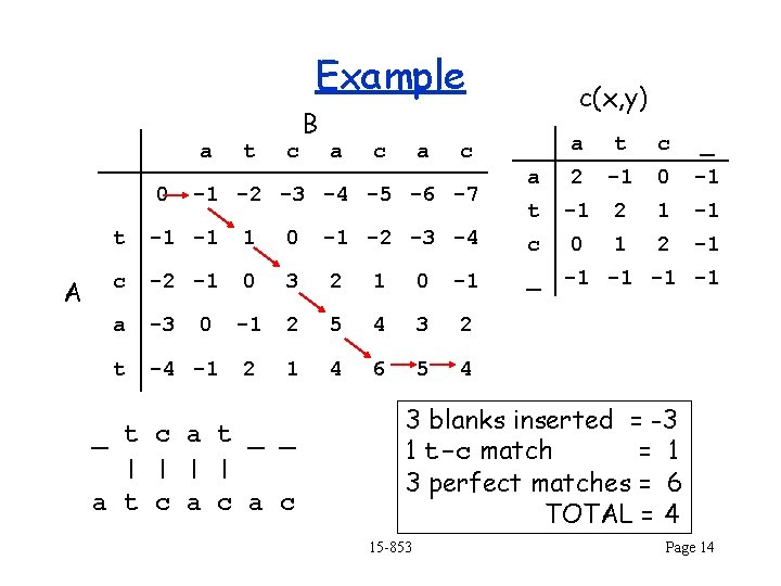
Example a 0 A t c B a c a a t c _ a 2 -1 0 -1 t -1 2 1 -1 c 0 1 2 -1 c -1 -2 -3 -4 -5 -6 -7 t -1 -1 1 0 c -2 -1 0 3 2 1 0 -1 a -3 0 -1 2 5 4 3 2 t -4 -1 2 1 4 6 5 4 _ t c a t _ _ | | a t c a c c(x, y) -1 -2 -3 -4 _ -1 -1 3 blanks inserted = -3 1 t-c match = 1 3 perfect matches = 6 TOTAL = 4 15 -853 Page 14

Optimizations Space efficiency: The divide-and-conquer technique still works. The Ukkonen/Myers algorithm: A variant works, but O(dn) time is no longer guaranteed since the distance from the diagonal cannot in general be directly bounded by the score. Bounds, however, can be given in terms of relative weights of matrix elements and the technique works reasonably well in practice. Real Problem: solves global-alignment problem when biologists care about the local-alignment problem. 15 -853 Page 15

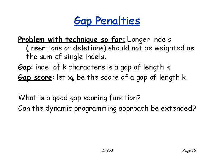
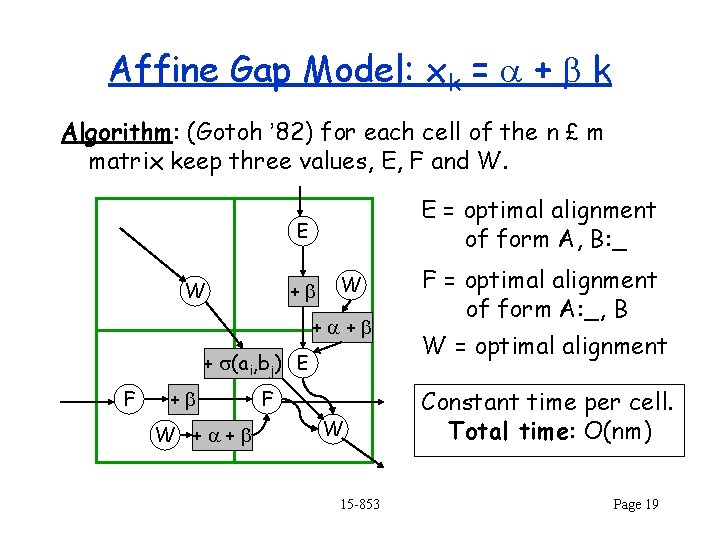
Gap Penalties Problem with technique so far: Longer indels (insertions or deletions) should not be weighted as the sum of single indels. Gap: indel of k characters is a gap of length k Gap score: let xk be the score of a gap of length k What is a good gap scoring function? Can the dynamic programming approach be extended? 15 -853 Page 16

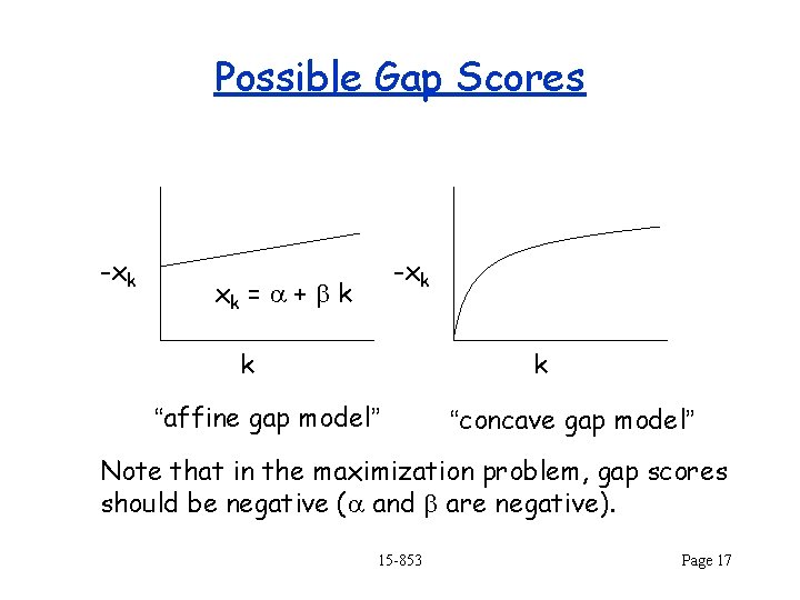
Possible Gap Scores -xk xk = a + b k k k “affine gap model” “concave gap model” Note that in the maximization problem, gap scores should be negative (a and b are negative). 15 -853 Page 17

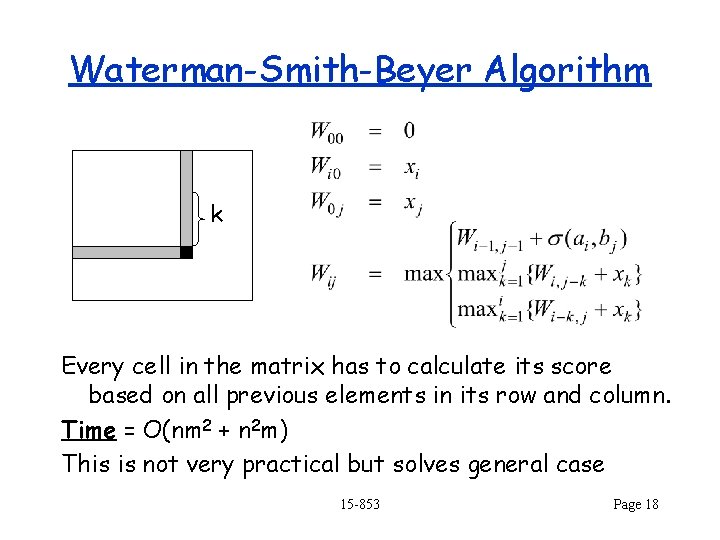
Waterman-Smith-Beyer Algorithm k Every cell in the matrix has to calculate its score based on all previous elements in its row and column. Time = O(nm 2 + n 2 m) This is not very practical but solves general case 15 -853 Page 18

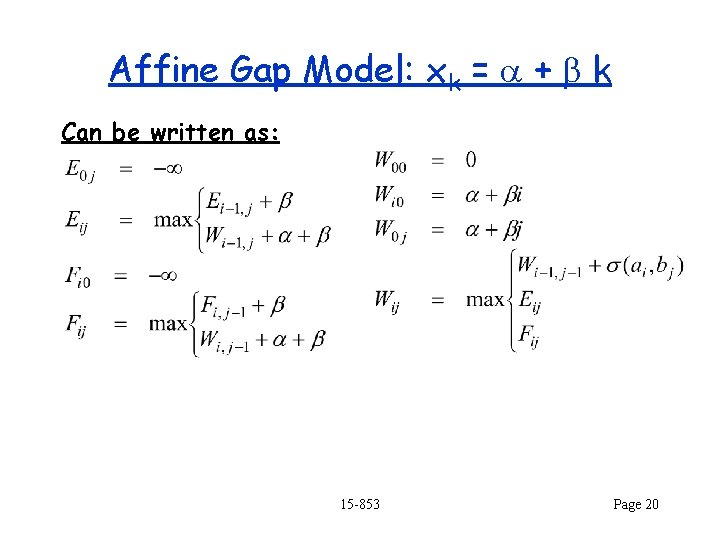
Affine Gap Model: xk = a + b k Algorithm: (Gotoh ’ 82) for each cell of the n £ m matrix keep three values, E, F and W. E = optimal alignment of form A, B: _ E W +b W +a+b + s(ai, bj) E F +b W +a+b F W 15 -853 F = optimal alignment of form A: _, B W = optimal alignment Constant time per cell. Total time: O(nm) Page 19

Affine Gap Model: xk = a + b k Can be written as: 15 -853 Page 20

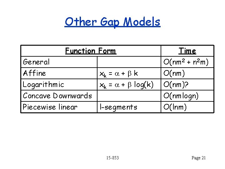
Other Gap Models Function Form General Affine Logarithmic xk = a + b k xk = a + b log(k) Concave Downwards Piecewise linear l-segments 15 -853 Time O(nm 2 + n 2 m) O(nm)? O(nmlogn) O(lnm) Page 21

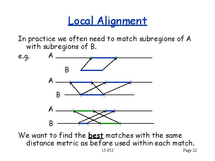
Local Alignment In practice we often need to match subregions of A with subregions of B. A e. g. B A B We want to find the best matches with the same distance metric as before used within each match. 15 -853 Page 22

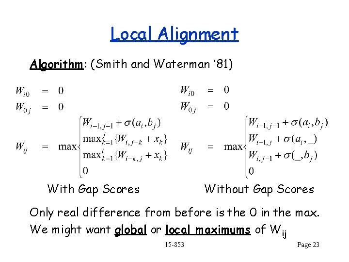
Local Alignment Algorithm: (Smith and Waterman ’ 81) With Gap Scores Without Gap Scores Only real difference from before is the 0 in the max. We might want global or local maximums of Wij 15 -853 Page 23

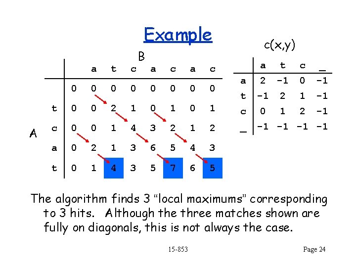
Example a A t c B a c(x, y) a t c _ a 2 -1 0 -1 t -1 2 1 -1 0 1 2 -1 c 0 0 0 0 t 0 0 2 1 0 1 c c 0 0 1 4 3 2 1 2 _ a 0 2 1 3 6 5 4 3 t 0 1 4 3 5 7 6 5 -1 -1 The algorithm finds 3 “local maximums” corresponding to 3 hits. Although the three matches shown are fully on diagonals, this is not always the case. 15 -853 Page 24

Example a 0 A t c B a c a a t c _ a 2 -1 0 -1 t -1 2 1 -1 c 0 1 2 -1 c -1 -2 -3 -4 -5 -6 -7 t -1 -1 1 0 c -2 -1 0 3 2 1 0 -1 a -3 0 -1 2 5 4 3 2 t -4 -1 2 1 4 6 5 4 _ t c a t _ _ | | a t c a c c(x, y) -1 -2 -3 -4 _ -1 -1 3 blanks inserted = -3 1 t-c match = 1 3 perfect matches = 6 TOTAL = 4 15 -853 Page 25

Database Search Basic model: 1. User selects a database and submits a source sequence S, typically via the web (or email) 2. The remote computer compares S to each target T in its database. The runtime depends on the length of S and the size of the database. 3. The remote computer returns a ranked list of the “best” hits found in the database, usually based on local alignment. Example of BLAST 15 -853 Page 26

Algorithms in the “real world” Dynamic programming is too expensive even with optimizations. Heuristics are used that approximate the dynamic programming solution. Dynamic program is often used at end to give final score. Main two programs in practice: – FASTA (1985) – BLAST (Basic Local Alignment Search Tool) (1990) Lipman involed in both, Myers involved in BLAST. There are many variants of both. 15 -853 Page 27

FASTA and BLAST The idea of both algorithms is to find approximate matches by composing smaller exact matches. Both algorithms loop over each string T in the database and find the “heuristically” best match for the search string along with its score (assuming the score is above some threshold). The matches across the T in the database are returned in rank order (highest-score first). 15 -853 Page 28

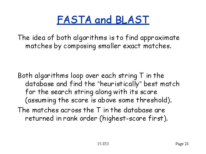
FASTA: Step 1 Break source S into k-tuples (adjacent sequence of k characters) using a “sliding window”. Typically k=1 or 2 for proteins, and k=4 -6 for DNA. S k Create a table that maps each k-tuple value found to all the start positions with that value 15 -853 Page 29

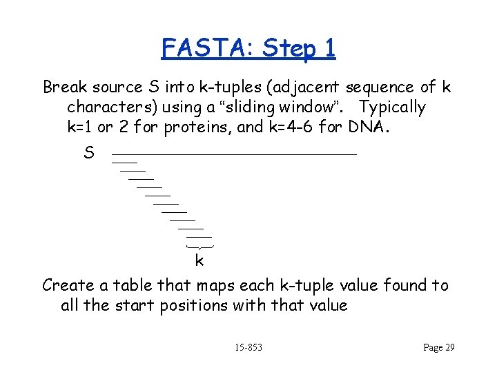
FASTA: Step 2 Linearly search T for each k-tuple belonging to S and bucket the hits (called “hot spots”) by diagonal. T S j At Tj there are two hits in the table giving positions i 1 and i 2 in S, which are in diagonals j - i 1 and j - i 2 i 1 i 2 k 15 -853 Page 30

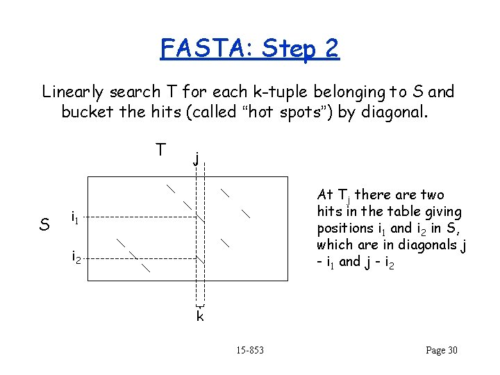
FASTA: Step 3 Join hits along diagonals into runs by 1. Each hit gets a positive score and each space between hits a negative score that increases with distance. 2. Finding runs that have maximal score (i. e. the sum of the scores cannot be increase by extending the run). There might be more than one such run in a diagonal. T S 15 -853 Page 31

FASTA: Step 4 Select top k (e. g. 10) scores from step 3, and rescore them using a substitution matrix (e. g. BLOSUM 62). The best score is called init 1. Any scores below a threshold is thrown out. This leaves between 0 and 10 runs. 15 -853 Page 32

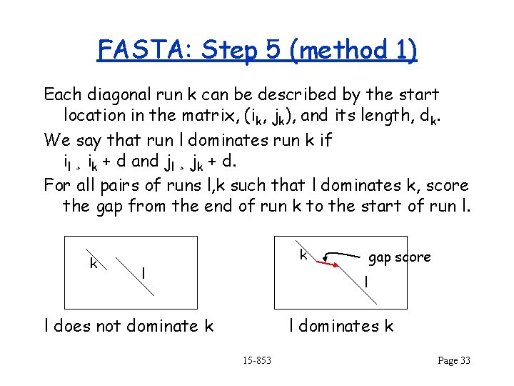
FASTA: Step 5 (method 1) Each diagonal run k can be described by the start location in the matrix, (ik, jk), and its length, dk. We say that run l dominates run k if il ¸ ik + d and jl ¸ jk + d. For all pairs of runs l, k such that l dominates k, score the gap from the end of run k to the start of run l. k k l gap score l l does not dominate k l dominates k 15 -853 Page 33

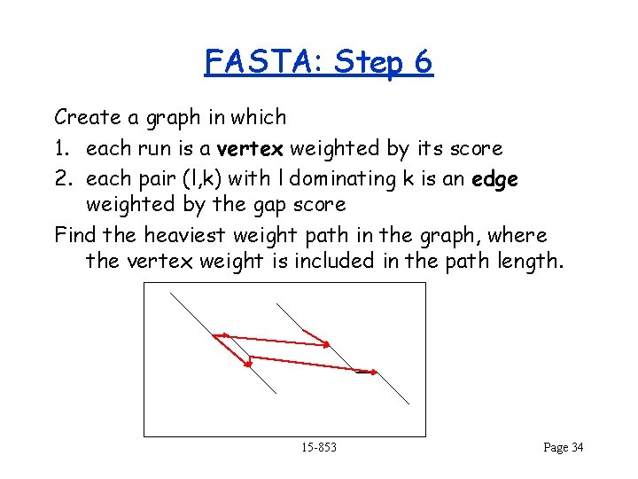
FASTA: Step 6 Create a graph in which 1. each run is a vertex weighted by its score 2. each pair (l, k) with l dominating k is an edge weighted by the gap score Find the heaviest weight path in the graph, where the vertex weight is included in the path length. 15 -853 Page 34

FASTA: Step 7 After the path is found, dynamic programming is used to give a more accurate score to the path. We now have a global alignment problem (since we know the start and end of each string), so we can use the Myers/Ukkonen algorithm. 15 -853 Page 35

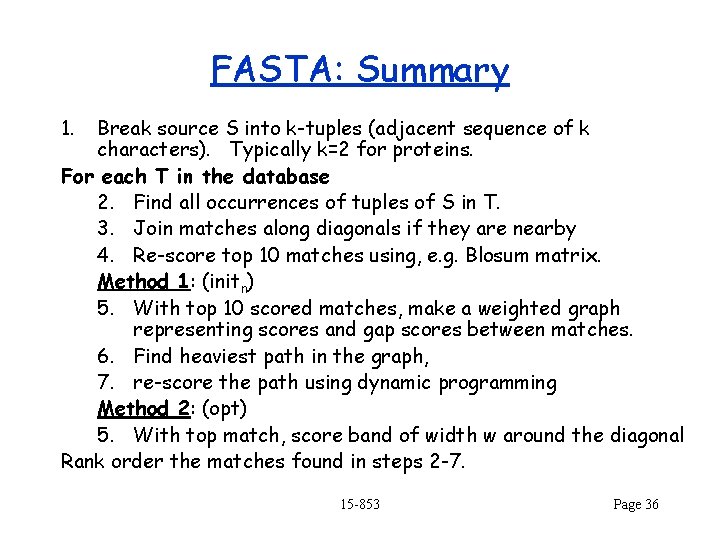
FASTA: Summary 1. Break source S into k-tuples (adjacent sequence of k characters). Typically k=2 for proteins. For each T in the database 2. Find all occurrences of tuples of S in T. 3. Join matches along diagonals if they are nearby 4. Re-score top 10 matches using, e. g. Blosum matrix. Method 1: (initn) 5. With top 10 scored matches, make a weighted graph representing scores and gap scores between matches. 6. Find heaviest path in the graph, 7. re-score the path using dynamic programming Method 2: (opt) 5. With top match, score band of width w around the diagonal Rank order the matches found in steps 2 -7. 15 -853 Page 36

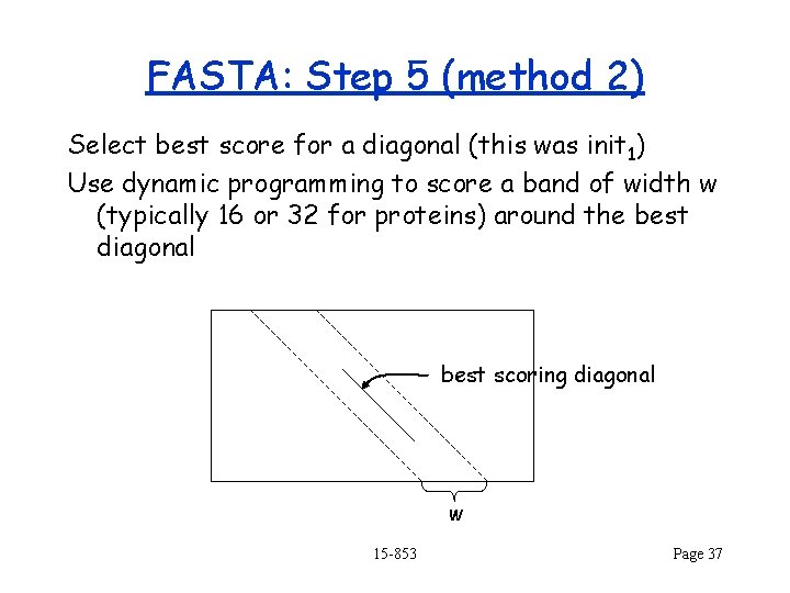
FASTA: Step 5 (method 2) Select best score for a diagonal (this was init 1) Use dynamic programming to score a band of width w (typically 16 or 32 for proteins) around the best diagonal best scoring diagonal w 15 -853 Page 37

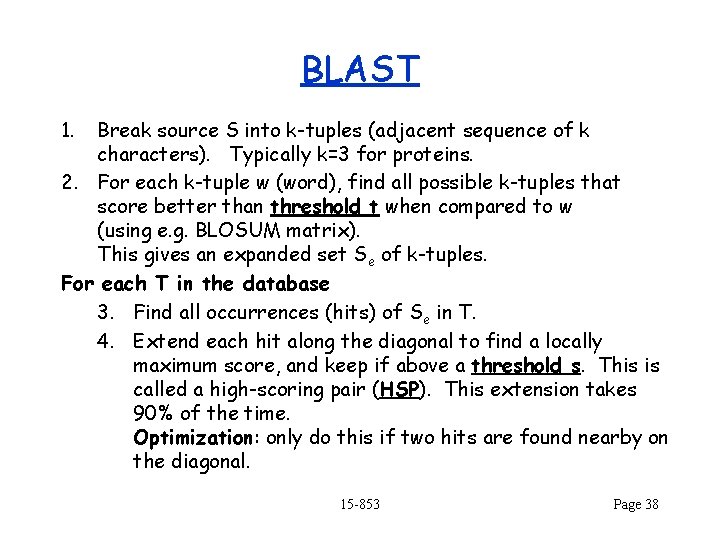
BLAST 1. Break source S into k-tuples (adjacent sequence of k characters). Typically k=3 for proteins. 2. For each k-tuple w (word), find all possible k-tuples that score better than threshold t when compared to w (using e. g. BLOSUM matrix). This gives an expanded set Se of k-tuples. For each T in the database 3. Find all occurrences (hits) of Se in T. 4. Extend each hit along the diagonal to find a locally maximum score, and keep if above a threshold s. This is called a high-scoring pair (HSP). This extension takes 90% of the time. Optimization: only do this if two hits are found nearby on the diagonal. 15 -853 Page 38

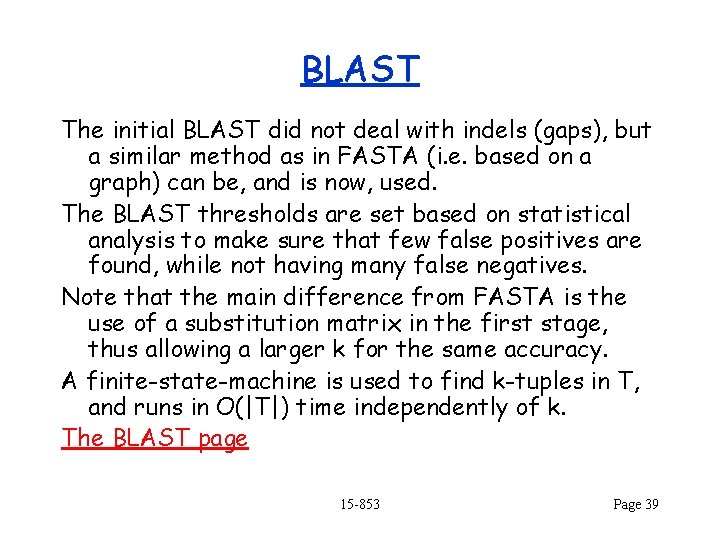
BLAST The initial BLAST did not deal with indels (gaps), but a similar method as in FASTA (i. e. based on a graph) can be, and is now, used. The BLAST thresholds are set based on statistical analysis to make sure that few false positives are found, while not having many false negatives. Note that the main difference from FASTA is the use of a substitution matrix in the first stage, thus allowing a larger k for the same accuracy. A finite-state-machine is used to find k-tuples in T, and runs in O(|T|) time independently of k. The BLAST page 15 -853 Page 39