15 853 Algorithms in the Real World Error

15 -853: Algorithms in the Real World Error Correcting Codes I – Overview – Hamming Codes – Linear Codes 15 -853 1

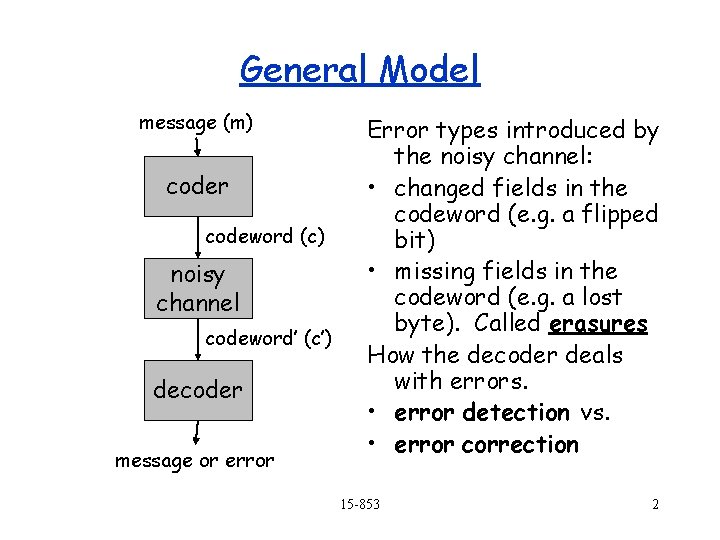
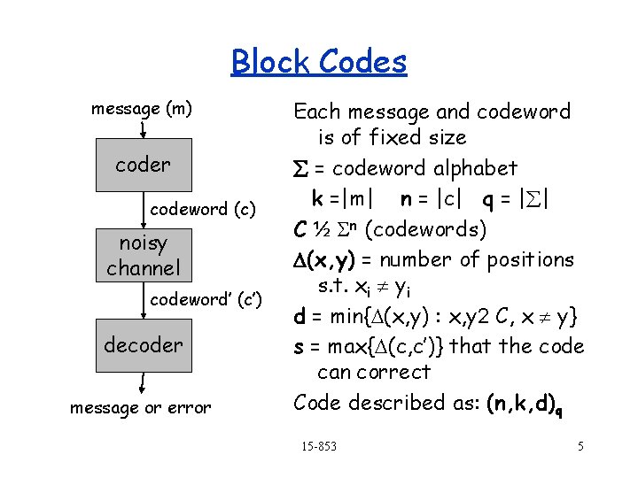
General Model message (m) coder codeword (c) noisy channel codeword’ (c’) decoder message or error Error types introduced by the noisy channel: • changed fields in the codeword (e. g. a flipped bit) • missing fields in the codeword (e. g. a lost byte). Called erasures How the decoder deals with errors. • error detection vs. • error correction 15 -853 2

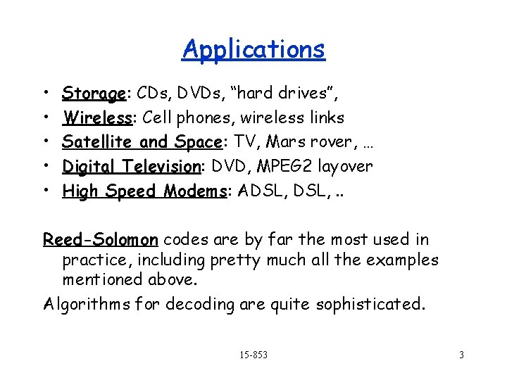
Applications • • • Storage: CDs, DVDs, “hard drives”, Wireless: Cell phones, wireless links Satellite and Space: TV, Mars rover, … Digital Television: DVD, MPEG 2 layover High Speed Modems: ADSL, . . Reed-Solomon codes are by far the most used in practice, including pretty much all the examples mentioned above. Algorithms for decoding are quite sophisticated. 15 -853 3

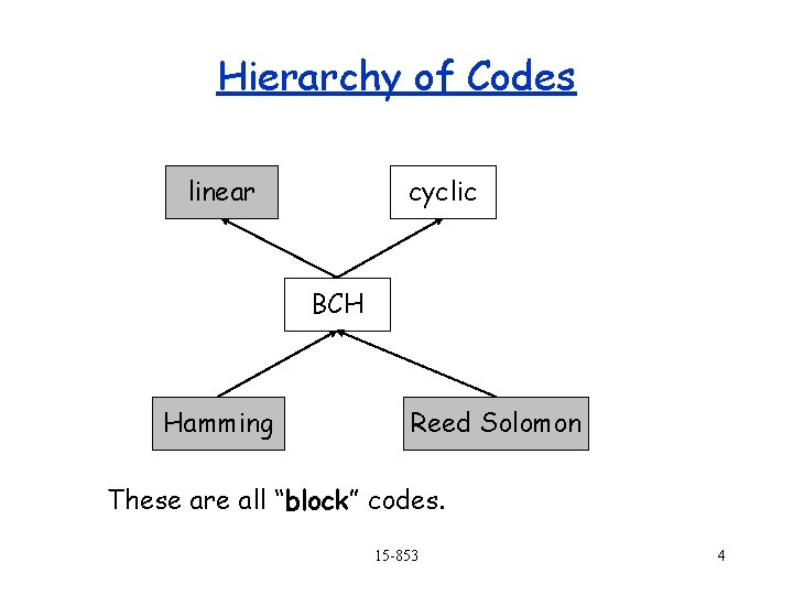
Hierarchy of Codes linear cyclic BCH Hamming Reed Solomon These are all “block” codes. 15 -853 4

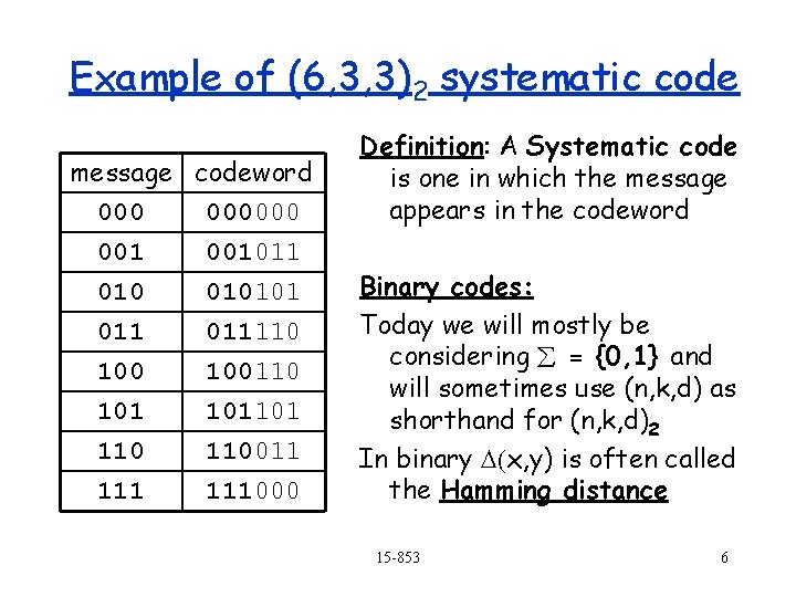
Block Codes message (m) coder codeword (c) noisy channel codeword’ (c’) decoder message or error Each message and codeword is of fixed size å = codeword alphabet k =|m| n = |c| q = |å| C ½ Sn (codewords) D(x, y) = number of positions s. t. xi ¹ yi d = min{D(x, y) : x, y 2 C, x ¹ y} s = max{D(c, c’)} that the code can correct Code described as: (n, k, d)q 15 -853 5

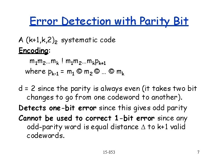
Example of (6, 3, 3)2 systematic code message codeword 000000 001011 010101 011 100 101 110 111 011110 100110 101101 110011 111000 Definition: A Systematic code is one in which the message appears in the codeword Binary codes: Today we will mostly be considering å = {0, 1} and will sometimes use (n, k, d) as shorthand for (n, k, d)2 In binary D(x, y) is often called the Hamming distance 15 -853 6

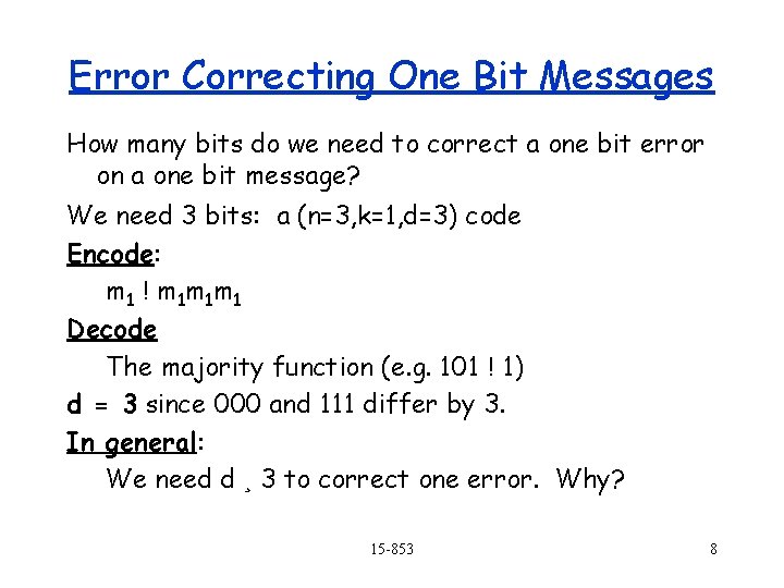
Error Detection with Parity Bit A (k+1, k, 2)2 systematic code Encoding: m 1 m 2…mk ! m 1 m 2…mkpk+1 where pk-1 = m 1 © m 2 © … © mk d = 2 since the parity is always even (it takes two bit changes to go from one codeword to another). Detects one-bit error since this gives odd parity Cannot be used to correct 1 -bit error since any odd-parity word is equal distance D to k+1 valid codewords. 15 -853 7

Error Correcting One Bit Messages How many bits do we need to correct a one bit error on a one bit message? We need 3 bits: a (n=3, k=1, d=3) code Encode: m 1 ! m 1 m 1 m 1 Decode The majority function (e. g. 101 ! 1) d = 3 since 000 and 111 differ by 3. In general: We need d ¸ 3 to correct one error. Why? 15 -853 8

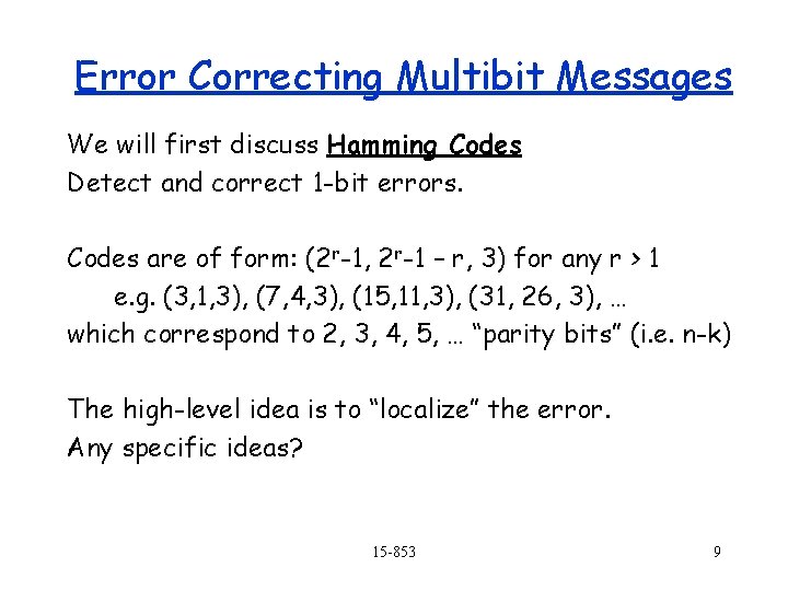
Error Correcting Multibit Messages We will first discuss Hamming Codes Detect and correct 1 -bit errors. Codes are of form: (2 r-1, 2 r-1 – r, 3) for any r > 1 e. g. (3, 1, 3), (7, 4, 3), (15, 11, 3), (31, 26, 3), … which correspond to 2, 3, 4, 5, … “parity bits” (i. e. n-k) The high-level idea is to “localize” the error. Any specific ideas? 15 -853 9

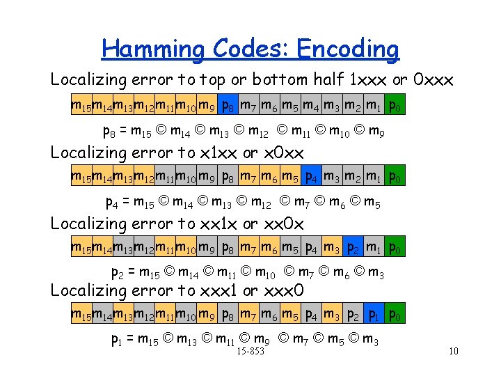
Hamming Codes: Encoding Localizing error to top or bottom half 1 xxx or 0 xxx m 15 m 14 m 13 m 12 m 11 m 10 m 9 p 8 m 7 m 6 m 5 m 4 m 3 m 2 m 1 p 0 p 8 = m 15 © m 14 © m 13 © m 12 © m 11 © m 10 © m 9 Localizing error to x 1 xx or x 0 xx m 15 m 14 m 13 m 12 m 11 m 10 m 9 p 8 m 7 m 6 m 5 p 4 m 3 m 2 m 1 p 0 p 4 = m 15 © m 14 © m 13 © m 12 © m 7 © m 6 © m 5 Localizing error to xx 1 x or xx 0 x m 15 m 14 m 13 m 12 m 11 m 10 m 9 p 8 m 7 m 6 m 5 p 4 m 3 p 2 m 1 p 0 p 2 = m 15 © m 14 © m 11 © m 10 © m 7 © m 6 © m 3 Localizing error to xxx 1 or xxx 0 m 15 m 14 m 13 m 12 m 11 m 10 m 9 p 8 m 7 m 6 m 5 p 4 m 3 p 2 p 1 p 0 p 1 = m 15 © m 13 © m 11 © m 9 © m 7 © m 5 © m 3 15 -853 10

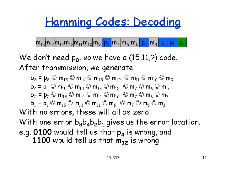
Hamming Codes: Decoding m 15 m 14 m 13 m 12 m 11 m 10 m 9 p 8 m 7 m 6 m 5 p 4 m 3 p 2 p 1 p 0 We don’t need p 0, so we have a (15, 11, ? ) code. After transmission, we generate b 8 = p 8 © m 15 © m 14 © m 13 © m 12 © m 11 © m 10 © m 9 b 4 = p 4 © m 15 © m 14 © m 13 © m 12 © m 7 © m 6 © m 5 b 2 = p 2 © m 15 © m 14 © m 11 © m 10 © m 7 © m 6 © m 3 b 1 = p 1 © m 15 © m 13 © m 11 © m 9 © m 7 © m 5 © m 3 With no errors, these will all be zero With one error b 8 b 4 b 2 b 1 gives us the error location. e. g. 0100 would tell us that p 4 is wrong, and 1100 would tell us that m 12 is wrong 15 -853 11

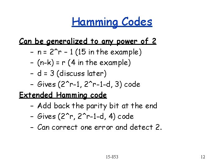
Hamming Codes Can be generalized to any power of 2 – n = 2^r – 1 (15 in the example) – (n-k) = r (4 in the example) – d = 3 (discuss later) – Gives (2^r-1, 2^r-1 -d, 3) code Extended Hamming code – Add back the parity bit at the end – Gives (2^r, 2^r-1 -d, 4) code – Can correct one error and detect 2. 15 -853 12

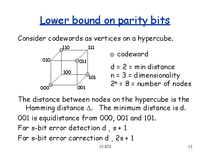
Lower bound on parity bits Consider codewords as vertices on a hypercube. 110 010 111 011 100 000 101 001 codeword d = 2 = min distance n = 3 = dimensionality 2 n = 8 = number of nodes The distance between nodes on the hypercube is the Hamming distance D. The minimum distance is d. 001 is equidistance from 000, 001 and 101. For s-bit error detection d ¸ s + 1 For s-bit error correction d ¸ 2 s + 1 15 -853 13

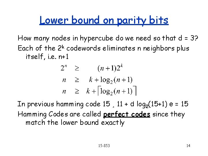
Lower bound on parity bits How many nodes in hypercube do we need so that d = 3? Each of the 2 k codewords eliminates n neighbors plus itself, i. e. n+1 In previous hamming code 15 ¸ 11 + d log 2(15+1) e = 15 Hamming Codes are called perfect codes since they match the lower bound exactly 15 -853 14

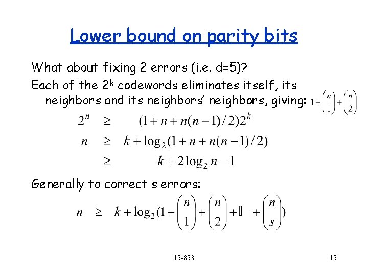
Lower bound on parity bits What about fixing 2 errors (i. e. d=5)? Each of the 2 k codewords eliminates itself, its neighbors and its neighbors’ neighbors, giving: Generally to correct s errors: 15 -853 15

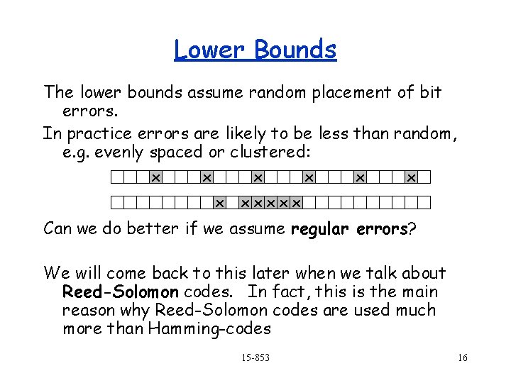
Lower Bounds The lower bounds assume random placement of bit errors. In practice errors are likely to be less than random, e. g. evenly spaced or clustered: x x x xxxxx Can we do better if we assume regular errors? We will come back to this later when we talk about Reed-Solomon codes. In fact, this is the main reason why Reed-Solomon codes are used much more than Hamming-codes 15 -853 16

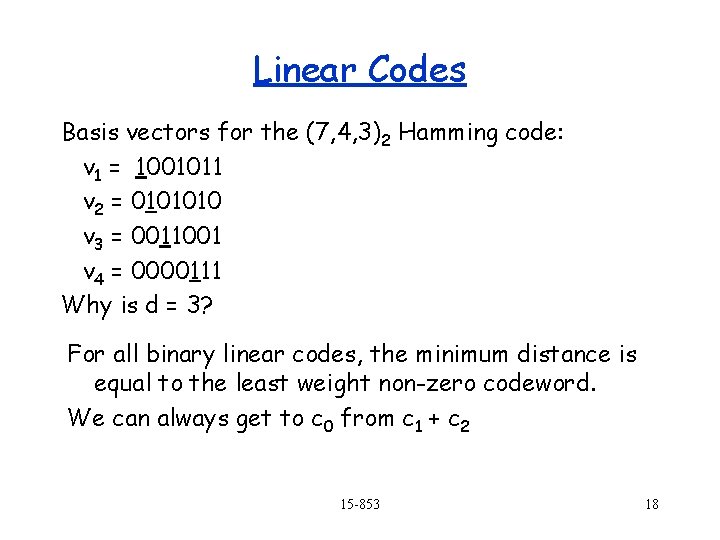
Linear Codes If å is a field, then ån is a vector space Definition: C is a linear code if it is a linear subspace of ån of dimension k. This means that there is a set of k basis vectors vi 2 ån (1 · i · k) that span the subspace. i. e. every code can be written as: c = a 1 v 1 + … + a k vk a i 2 å 15 -853 17

Linear Codes Basis vectors for the (7, 4, 3)2 Hamming code: v 1 = 1001011 v 2 = 0101010 v 3 = 0011001 v 4 = 0000111 Why is d = 3? For all binary linear codes, the minimum distance is equal to the least weight non-zero codeword. We can always get to c 0 from c 1 + c 2 15 -853 18

Generator and Parity Check Matrices Generator Matrix: A k x n matrix G such that: C = {x. G | x 2 åk} Made from stacking the basis vectors Parity Check Matrix: A (n – k) x n matrix H such that: C = {y 2 ån | Hy. T = 0} Codewords are the nullspace of H These always exist for linear codes HGT = 0 since: 0 = Hy. T = H(x. G)T = H(GTx. T) = (HGT)x. T only true for all x if HGT = 0 15 -853 19

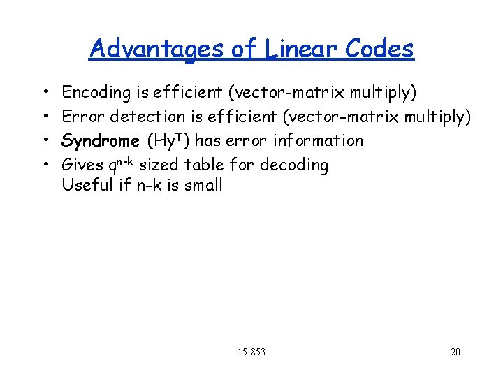
Advantages of Linear Codes • • Encoding is efficient (vector-matrix multiply) Error detection is efficient (vector-matrix multiply) Syndrome (Hy. T) has error information Gives qn-k sized table for decoding Useful if n-k is small 15 -853 20

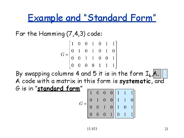
Example and “Standard Form” For the Hamming (7, 4, 3) code: By swapping columns 4 and 5 it is in the form Ik, A. A code with a matrix in this form is systematic, and G is in “standard form” 15 -853 21

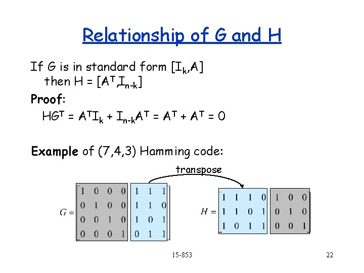
Relationship of G and H If G is in standard form [Ik, A] then H = [AT, In-k] Proof: HGT = ATIk + In-k. AT = AT + AT = 0 Example of (7, 4, 3) Hamming code: transpose 15 -853 22

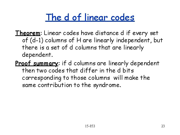
The d of linear codes Theorem: Linear codes have distance d if every set of (d-1) columns of H are linearly independent, but there is a set of d columns that are linearly dependent. Proof summary: if d columns are linearly dependent then two codes that differ in the d bits corresponding to those columns will make the same contribution to the syndrome. 15 -853 23

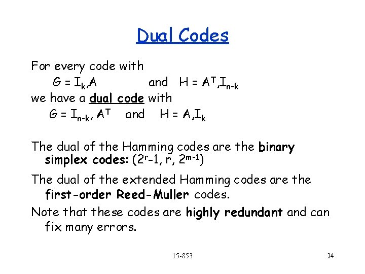
Dual Codes For every code with G = Ik, A and H = AT, In-k we have a dual code with G = In-k, AT and H = A, Ik The dual of the Hamming codes are the binary simplex codes: (2 r-1, r, 2 m-1) The dual of the extended Hamming codes are the first-order Reed-Muller codes. Note that these codes are highly redundant and can fix many errors. 15 -853 24

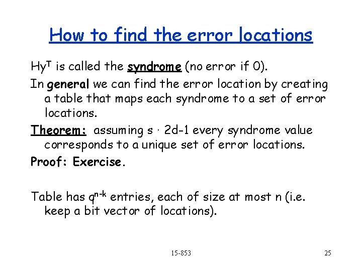
How to find the error locations Hy. T is called the syndrome (no error if 0). In general we can find the error location by creating a table that maps each syndrome to a set of error locations. Theorem: assuming s · 2 d-1 every syndrome value corresponds to a unique set of error locations. Proof: Exercise. Table has qn-k entries, each of size at most n (i. e. keep a bit vector of locations). 15 -853 25